
Concept | Time series extrema extraction#
Watch the video or read the summary below.
When working with time series data, we’re often particularly interested in what happens around their peaks or the bottom of their valleys.
More formally, across an entire time series, we can call the largest value the global maximum, and the smallest value the global minimum.
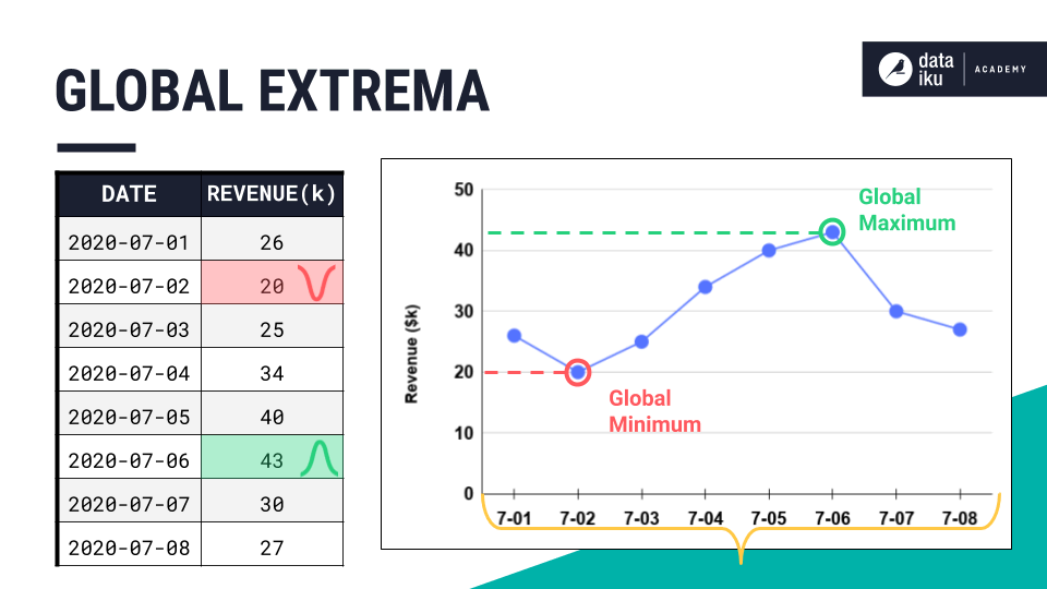
Together, we’d call these two points the global extrema of the time series.
Finding global extrema in Dataiku#
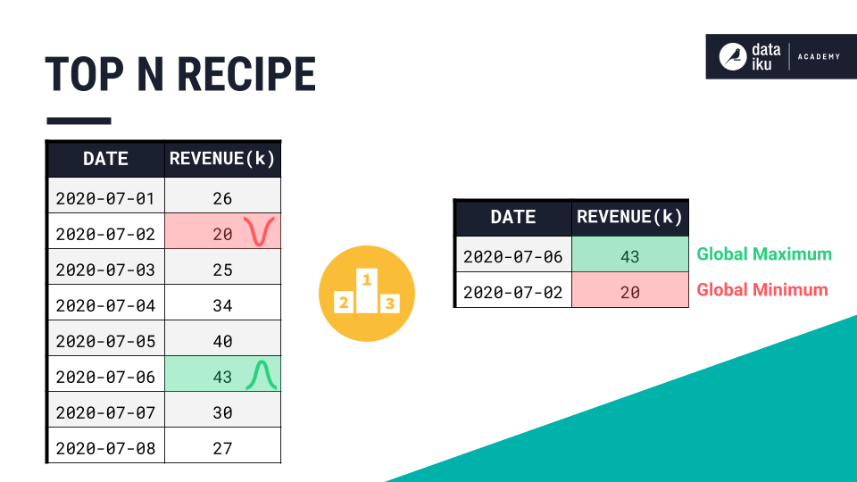
You probably already know a few ways to find the global extrema of a dataset in Dataiku. For example, we could use the Top N recipe to find any number of the largest or smallest values in the series.
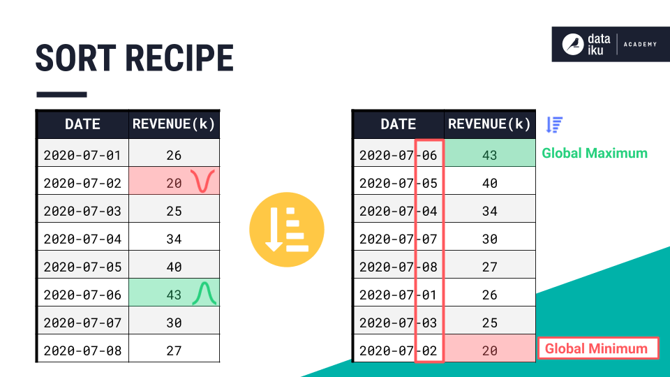
Alternatively, we could use the Sort recipe to order all values in the series by any column. But as we’ve said before, time series aren’t independent observations. Just sorting by the magnitude of values would mix up the chronological order of the time series.
Quite often though, we want to investigate not only the global extrema themselves, but also the points near them. For example, what can we learn from the data leading up to the global maximum? Or those immediately following it?

Extrema extraction use case#
As an example, imagine we have data coming from a car engine that we’re testing during the manufacturing process. In addition to knowing the car’s top velocity (the global maximum) on a test run, we might want to investigate metrics leading up to that peak moment.
For example, if the engine brakes, and velocity reaches a global minimum of 0, we might want to investigate metrics along its downward trajectory. In these kinds of cases, we essentially want to build “windows” around our global extrema.

Time series windowing#
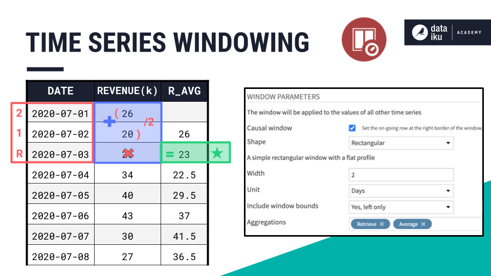
Luckily, we have a windowing recipe in the time series preparation plugin! In discussing the Time Series Windowing recipe, we described how to define window frames using parameters for causality, shape, width, units, and bounds.
Using those window frames, we then calculated rolling aggregations like sums and averages for each row of the dataset.
The same Window Parameters section, found in the Time Series Windowing recipe, is also found in the extrema extraction recipe.

You can therefore build on your knowledge of defining window frames when you work with the Extrema Extraction recipe!
Windowing with the extrema extraction recipe#
However, note that while the Windowing recipe calculates rolling aggregations on every row in our data, the Extrema Extraction recipe, calculates aggregations only for a window of data around the global minimum or the global maximum in a column of our choice.

Extrema extraction walkthrough#
Let’s walk through a simple example.
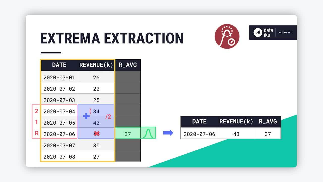
Using the time series windowing recipe, we could define a causal, rectangular window frame of two days, including only the left bound. Then we’d be able to calculate a rolling average sliding down this window frame.
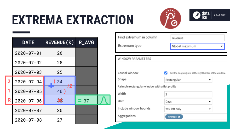
We can define a window frame of the same size with the extrema extraction recipe. But, we have two additional parameters to specify:
The type of extremum.
The column where it should be found.
The recipe then finds the chosen extremum–here, a global maximum on the revenue column.
For a causal window, as is the case in this example, our extremum serves as the right bound of the window. From the right bound, we draw the window frame according to the width, as we normally would.
Because we’ve excluded the right bound from the aggregation, only the values of the previous two days are included in the specified aggregation (an average).
Unlike the windowing recipe, which finds aggregations for a rolling window across every row in the data, here we’re calculating the aggregations only for the window around the extremum.
For a non-causal window, the process is the same, but the extremum would be the midpoint of the window. No matter the kind of window, for each time series in your dataset, the recipe returns only the row of the chosen extremum with the requested aggregation.
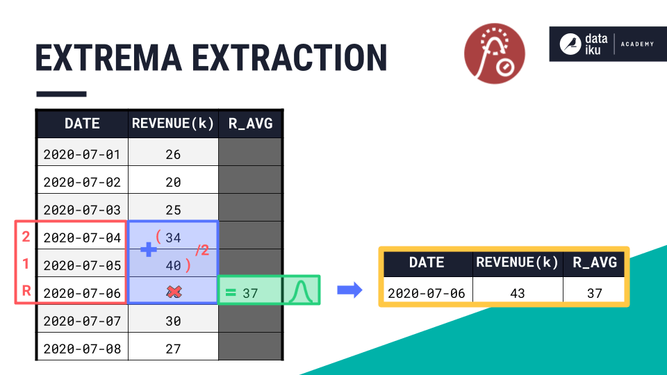
Let’s stay with this output for a moment. Because we have only a single time series, and there is a clear choice of extremum (no ties among the top values), we have only one output row. The aggregation column, in this output row, however, is able to draw on values from the chosen window frame.
Multiple time series#
What if we had multiple time series in the dataset and it was and it was stored in long format?
The extrema extraction recipe finds the extremum for each time series. If we have two time series in the dataset, the extrema extraction recipe will find two global maxima or two global minima and build the window frame accordingly around those points.
Extrema extraction in Dataiku#
We can see how this works with a demonstration on the resampled, long format orders dataset. We know the orders dataset contains six different time series, one for each product category.
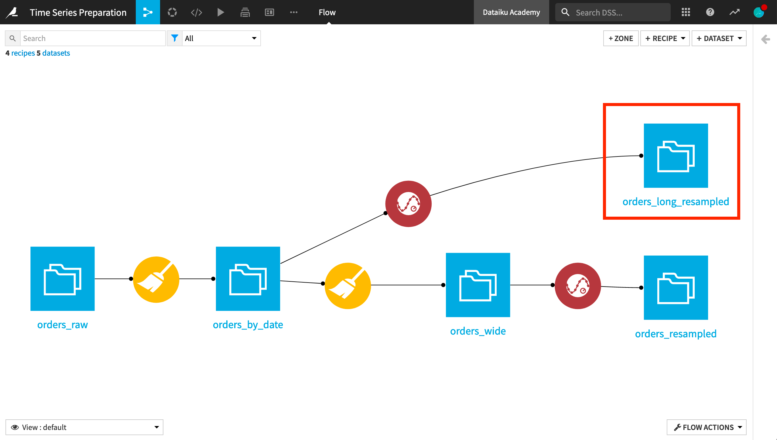
Let’s use the extrema extraction recipe to find the average amount spent in the week leading up to the global maximum.
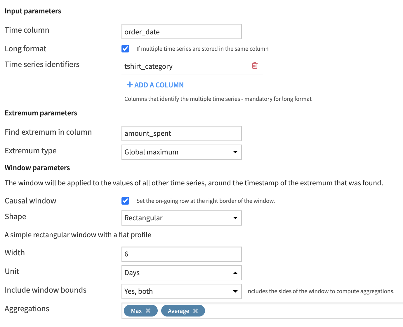
We’ll set order_date as the timestamp column.
We’re looking for the extremum in the column amount_spent.
Let’s select the global maximum as the extremum.
Let’s build a causal, rectangular window of six days, and include the left and right bounds. This means that the global maximum of each time series will be the right bound of the window.
Let’s calculate the average. Then, to check our work, we’ll also return the maximum.
Because we have multiple time series in long format, we need to provide the identifier column tshirt_category.
Let’s examine the output. We have the original four columns and four new columns. Our two columns of values each have two new columns of aggregations.
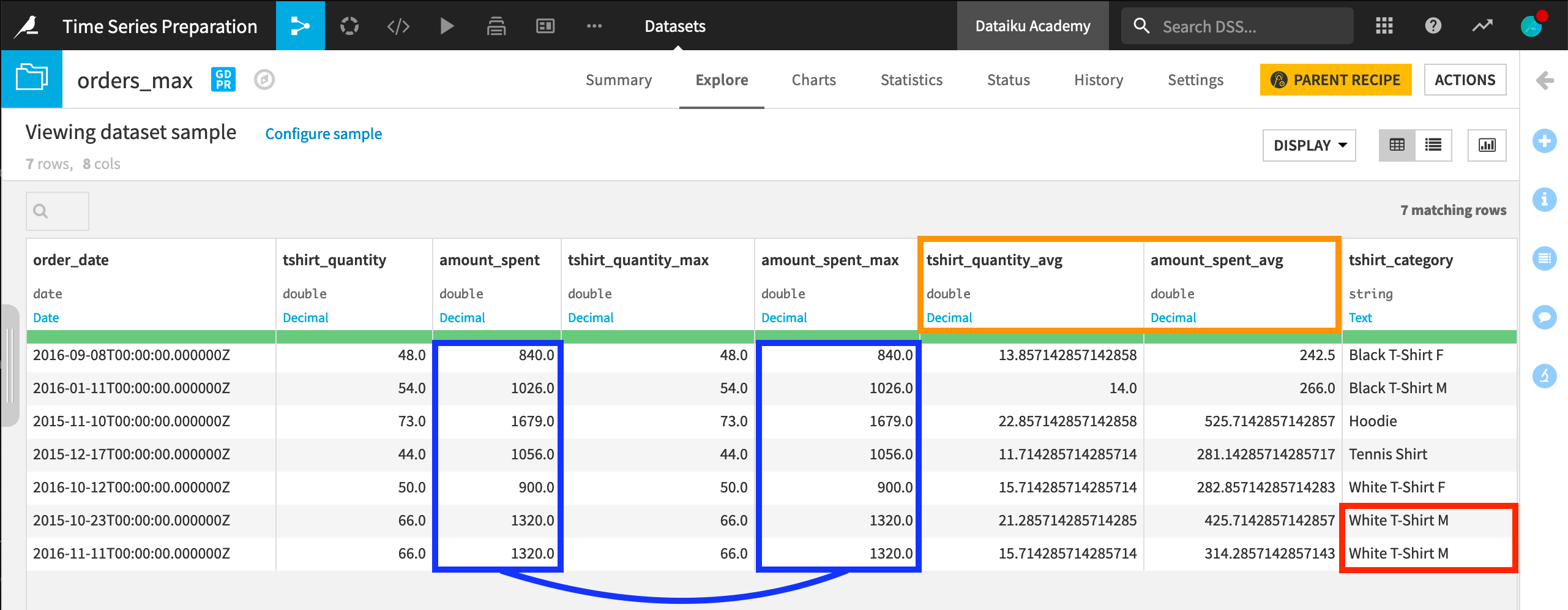
The maximum of amount_spent is the same as the original column. This makes sense because we wanted the recipe to find the global maximum in this column.
The average of amount_spent reflects the average of the global maximum, the right bound, and the previous six days.
We should also draw attention to the column tshirt_quantity. This dataset is an example of a multivariate time series because we have two columns of measurements for every timestamp. We built the window frame around the extremum in the amount_spent column, but the recipe returns the grouped aggregations for all numerical columns, and so we also get aggregations for the column tshirt_quantity too.
Finally, note that this dataset includes six different time series, but we have seven output rows. This is because two rows share the same global maximum for the white, male t-shirt category.
Next steps#
You are now ready to start building windows around extrema in your own time series datasets.
Try this recipe out for yourself in the next tutorial!