
Tutorial | Time series forecasting (visual ML)#
Get started#
Machine learning problems often involve a time component. This temporal constraint introduces complexities that require careful analysis.
Dataiku offers various ways to implement time series modeling and forecasting. This tutorial will focus on Dataiku’s time series analysis functionality within the visual machine learning interface.
Objectives#
In this tutorial, you will:
Design a time series forecasting model using the visual ML interface.
Train and deploy a forecasting model to the Flow.
Use the Evaluate and Score recipes with a forecasting model.
Prerequisites#
Dataiku 14.2 or later.
An Advanced Analytics Designer or Full Designer user profile.
Basic knowledge of visual ML in Dataiku (ML Practitioner level or equivalent).
If not using Dataiku Cloud (where it’s available by default), you’ll need a specific code environment including the required packages. See Runtime and GPU support in the reference documentation.
Note
If you want to perform some exploratory data analysis (EDA) before starting this forecasting project, visit Tutorial | Time series analysis.
Create the project#
From the Dataiku Design homepage, click + New Project.
Select Learning projects.
Search for and select Visual Time Series Forecasting.
If needed, change the folder into which the project will be installed, and click Create.
From the project homepage, click Go to Flow (or type
g+f).
Note
You can also download the starter project from this website and import it as a ZIP file.
You’ll next want to build the Flow.
Click Flow Actions at the bottom right of the Flow.
Click Build all.
Keep the default settings and click Build.
Use case summary#
The train dataset is a multivariate time series dataset that includes important columns:
Column |
Description |
|---|---|
product |
The category of the sold product: laptop, toy, and tshirt. |
date |
Daily sales of each product. |
sales |
The sales amount. |
is_holiday_flag |
A boolean flag that checks if the day is a holiday. |
website_traffic |
The amount of users going on the market website. |
promotion_level |
The discount rate applied. |
Design a forecasting model#
To build a time series model, you’ll use the train dataset. This dataset contains all time series data before 2024.
Tip
You’ll use the remaining time series values (occurring on 2024) as a validation set to evaluate the performance of your trained model.
Create the time series forecasting task#
The process is similar to that of other visual models.
From the Flow, select the train dataset, and navigate to the Lab (
 ) tab of the right panel.
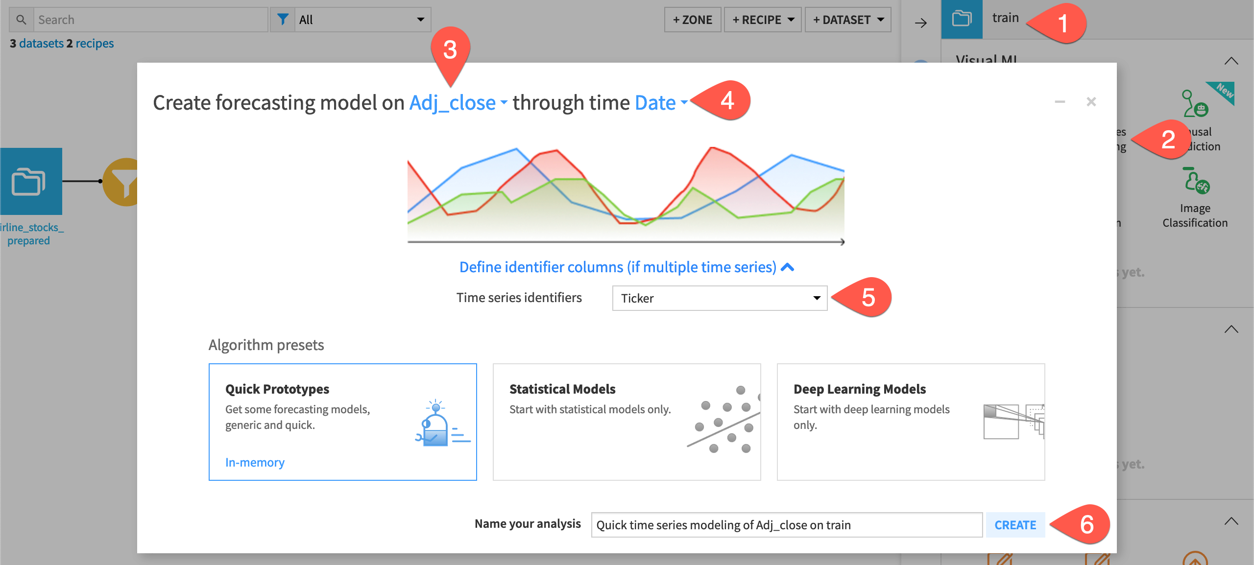
From the Visual ML section, select Time Series Forecasting.
Select sales as the numerical feature to forecast.
Select date as the date feature.
Under Define identifier columns, select product as the identifier column for the different time series.
Leaving the default for quick prototypes, click Create.
Configure the model’s general settings#
In the General settings panel of the Design tab, Dataiku has already specified parameter values based on:
The input selections from the forecasting task’s creation
The default settings
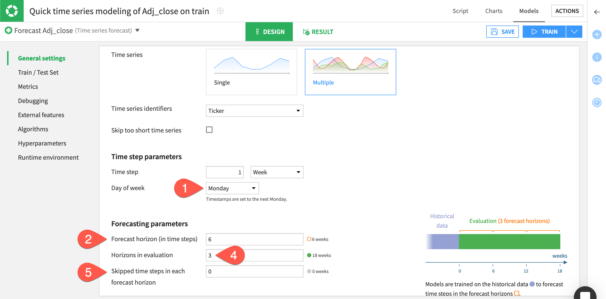
Let’s tweak these settings. This exercise aims at predicting the daily sales amount for the next 7 days and refresh the model every 28 days. Therefore, you’ll want to use an evaluation period of 28 days, equivalent to four forecast horizons.
Within the General settings panel of the modeling task’s Design tab, set the Time step to
1 Day.Under Forecasting parameters, set Forecast horizon (in time steps) to
7.Note
This parameter determines the length of the model forecast, so you should specify a value that’s a factor of the length of the validation set.
In the Changing forecast horizon window, select Re-detect settings.
Leave Skipped time steps in each forecast horizon at the default setting of
0. This parameter tells Dataiku the number of time steps within each horizon that you want to skip during the evaluation.
Configure the Train / Test Set panel#
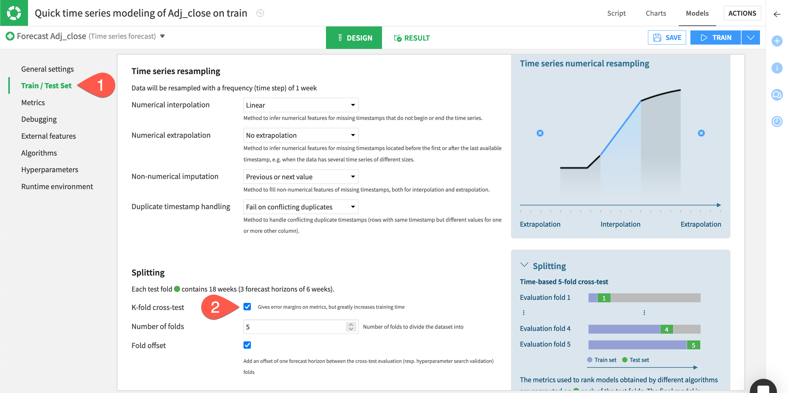
Because time series have an order, splitting in the train and test sets is quite different from a traditional machine learning problem.
In the Design tab, navigate to the Train / Test Set panel on the left.
In the Train/Test splitting section, leave the Auto setting by default.
Note
If you want to control the splitting, you can also click Custom and specify the date range you wish to have in your train and test folds.
Enter
4in the Horizons in test set field.Check the box for a K-fold cross-test splitting strategy, and keep the default of
5folds.
Note
Learn more about the K-fold cross-test by visiting Cross-validation.
Configure the Metrics panel#
The settings defined in the Metrics, Algorithms, and Hyperparameters panels define how Dataiku performs the search for the best model hyperparameters.
In the Metrics panel, you can choose the metric that Dataiku will use for model evaluation on the train and test sets.
On the left, navigate to the Metrics panel.
Switch to Mean Absolute Percentage Error (MAPE) as the metric for which the model’s hyperparameters should be optimized.
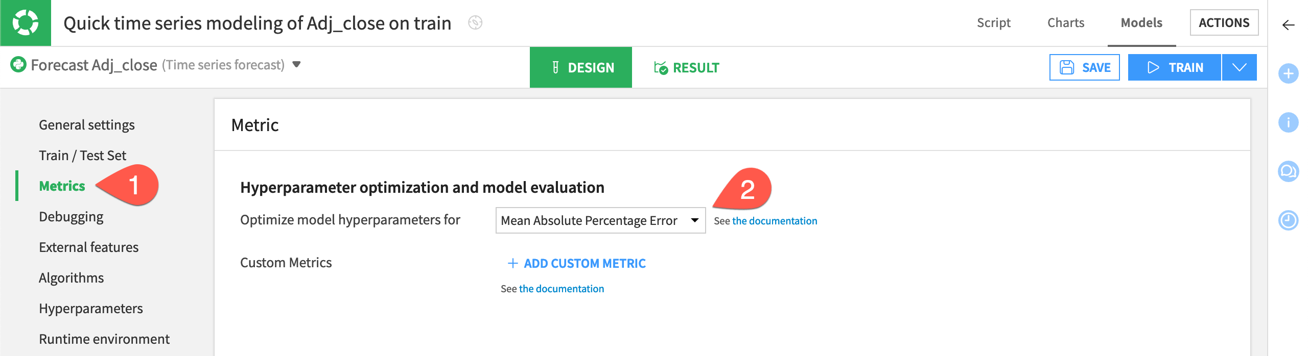
You can also click + Add Custom Metric to leverage business-related metric you could have.
Configure the External Features panel#
External features are exogenous time-dependent features. By default, Dataiku disables the external features for several reasons. One reason is that some training algorithms don’t support the use of external features.
In the present use case, external features can be relevant. Having past data to compute the impact of an event, or both past and future data to account for known events such as holidays or discounts, can improve predictions. Also, it’s recommended to have external features if you want to use classical machine learning techniques such as XGBoost or random forest that can lead to appealing results.
Navigate to the External features panel.
Check is_holiday_flag and promotion_level to enable multiple selection.
Select Input (past and future).
Select the past only parameter for website_traffic.
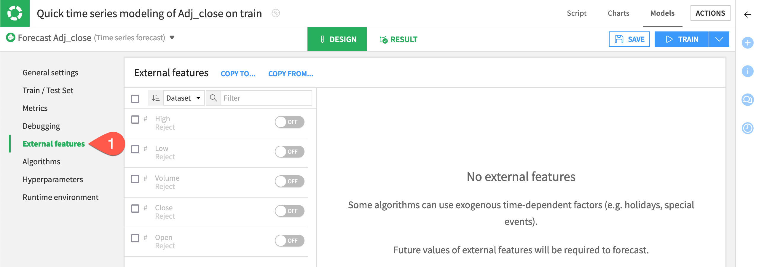
Holidays and promotions are features that can be known in advance and impact future sales, whereas website traffic is unknown in advance. These settings are relevant for this use case.
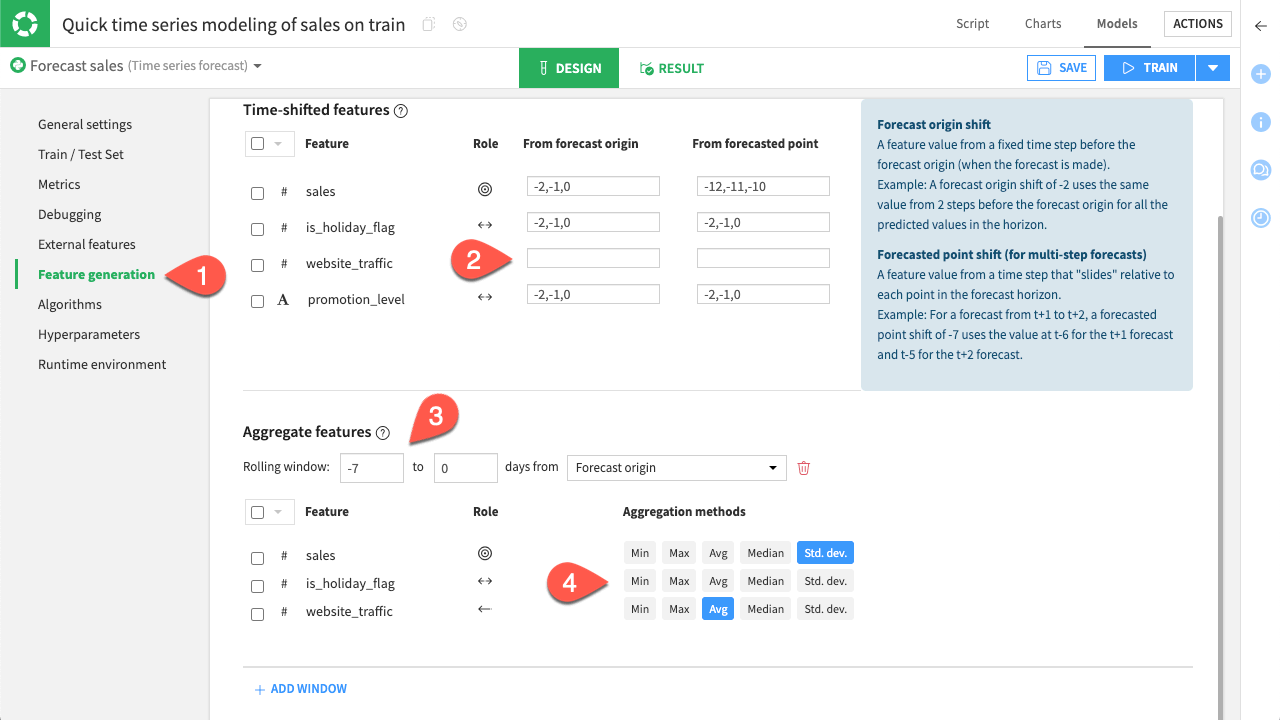
Generate new features#
The variables you selected as external features are now available for use. You can configure how you want new features to be generated from them.
For the time-shifted features, you have two choices:
Option |
Description |
|---|---|
From forecast origin |
The shift will start from the beginning of the horizon whatever the time step predicted. |
From the forecasted point |
The shift will start from the predicted time step. You’ll have to set a shift that is at least the number of time steps within the horizon. |
The second type of feature that you can generate is a window. With windows, you can aggregate past values of a feature to create a fixed historical value. For example, you can use the average web traffic over a week as a single feature that provides useful context.
Navigate to the Feature Generation panel.
Delete the From forecast origin input in website_traffic, so that no feature is created from it.
Set the default rolling window of
-7, as it represents the weekly window you need.For the aggregation methods, only select:
Std. dev. for sales, and
Avg for website_traffic.
See also
For more information, see the Shifts and Automatic shift selection sections in the reference documentation.
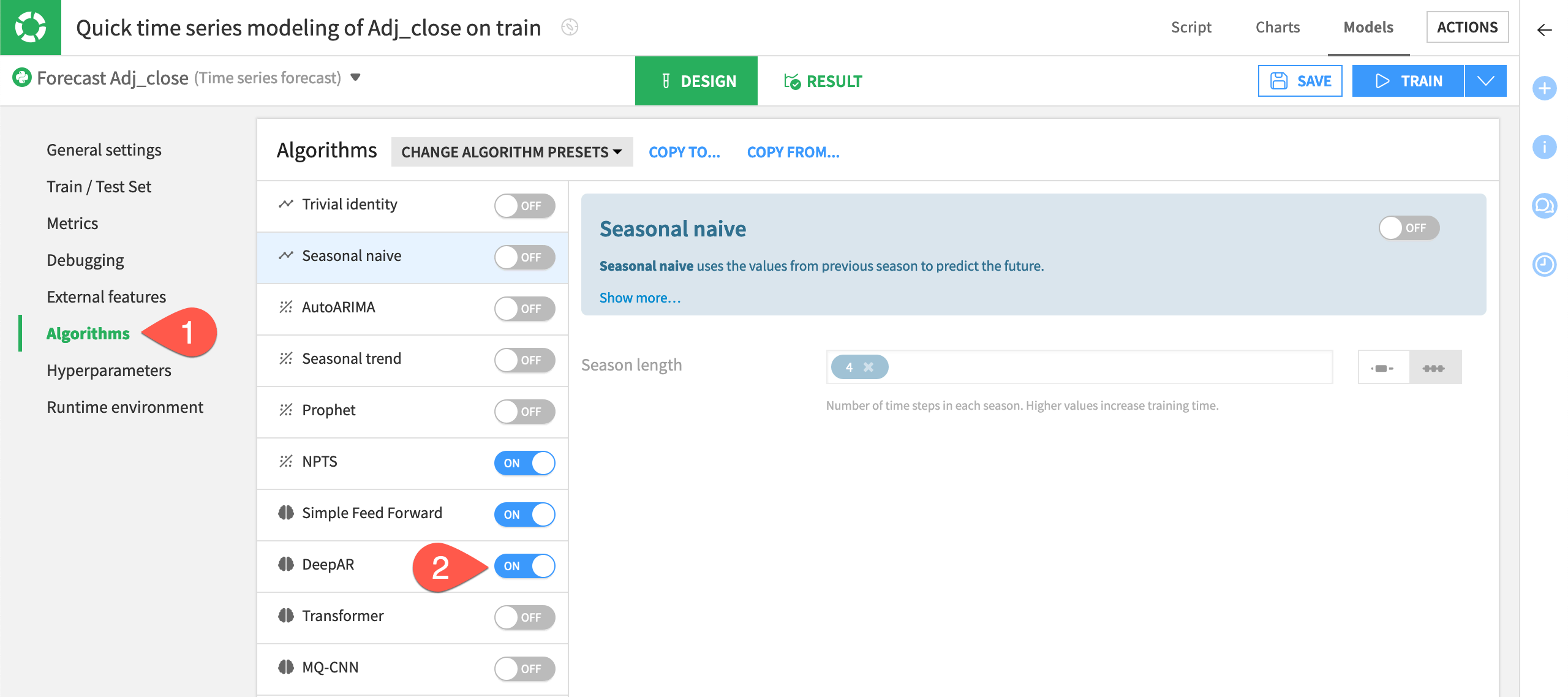
Configure the Algorithms panel#
The visual ML interface offers four categories of forecasting algorithms as indicated by the icon to the right of their names: statistical, deep learning, classical ML, and baseline.
During the hyperparameters optimization phase, Dataiku will evaluate each set of hyperparameters (defined in the Algorithms page) with the metric defined in the Metrics page.
On the left, navigate to the Algorithms panel.
In addition to the default selections based on the quick prototype designation, add the DeepAR - Torch and XGBoost algorithms, under Deep learning and Classical ML, respectively.
Deselect Ridge Regression under Classical ML.
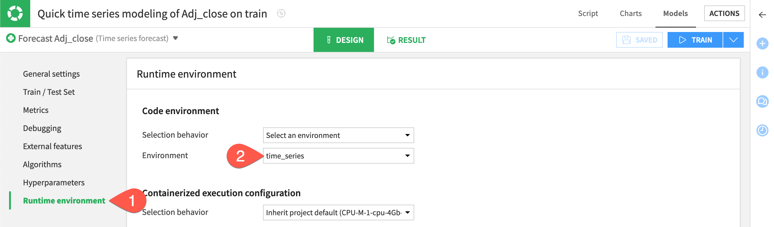
Inspect the Runtime environment#
One last step before training is to confirm that you have a compatible code environment in place.
On the left, navigate to the Runtime environment panel.
If not already present, select a code environment that includes the required packages for time series forecasting models.
Train and deploy a forecasting model#
Once you’re satisfied with the model’s design, you can go ahead training a session of models, and then choosing one to deploy to the Flow. You’ll notice that this process is the same for any other visual prediction or clustering model.
Train time series forecasting models#
Let’s kick off the training session!
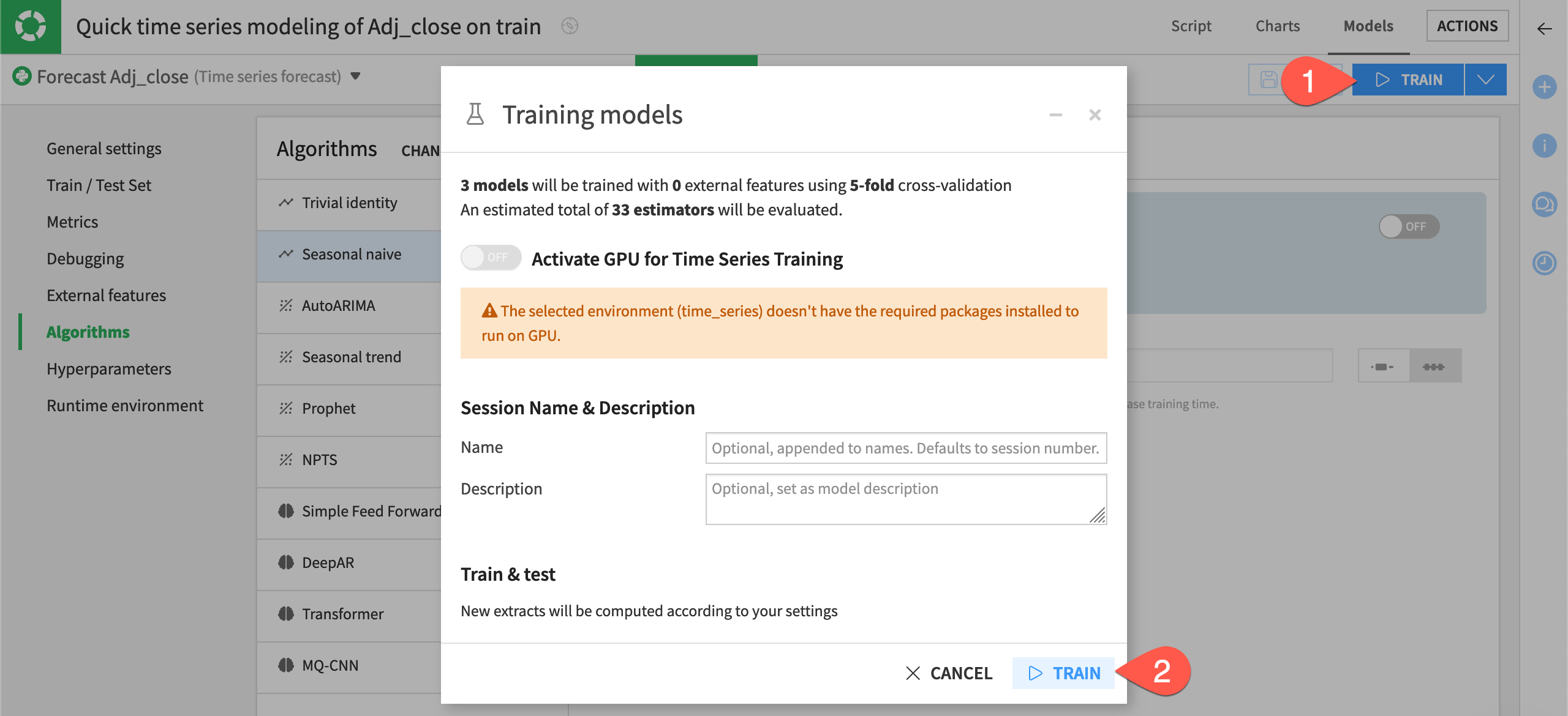
Near the top right of the modeling task, click Train.
In the dialog, click Train once more to start the training session.
Inspect the training results#
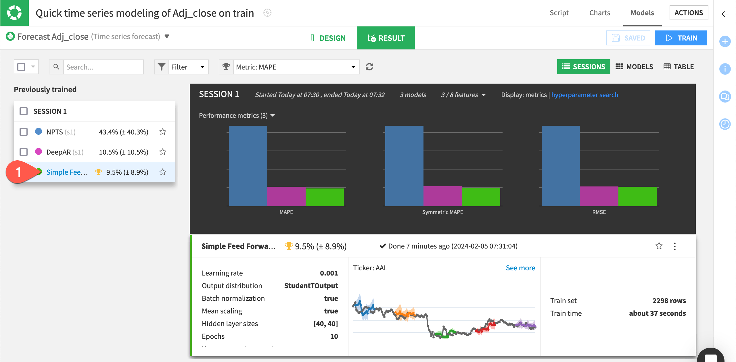
The bar charts at the top allow you to compare different metrics across the trained models. In this case, the XGBoost algorithm performed best for all three metrics (MAPE, Symmetric MAPE, and RMSE).
Tip
Click the Metrics dropdown on top of the session summary to change the displayed metrics.
On the left of the Result tab, click the best-performing model, XGBoost, to see the model training results.
In the Report tab, click on Metrics to have an overview of all the metrics in which your model has performed.
As for other visual models, the model report provides a number of visualizations and metrics related to the model’s performance.
Still in the Report tab, navigate to the Metrics per time series.
Under Per-fold metrics, toggle On the option.
Notice the different performance metrics of your model for each of the folds set up for cross-validation.
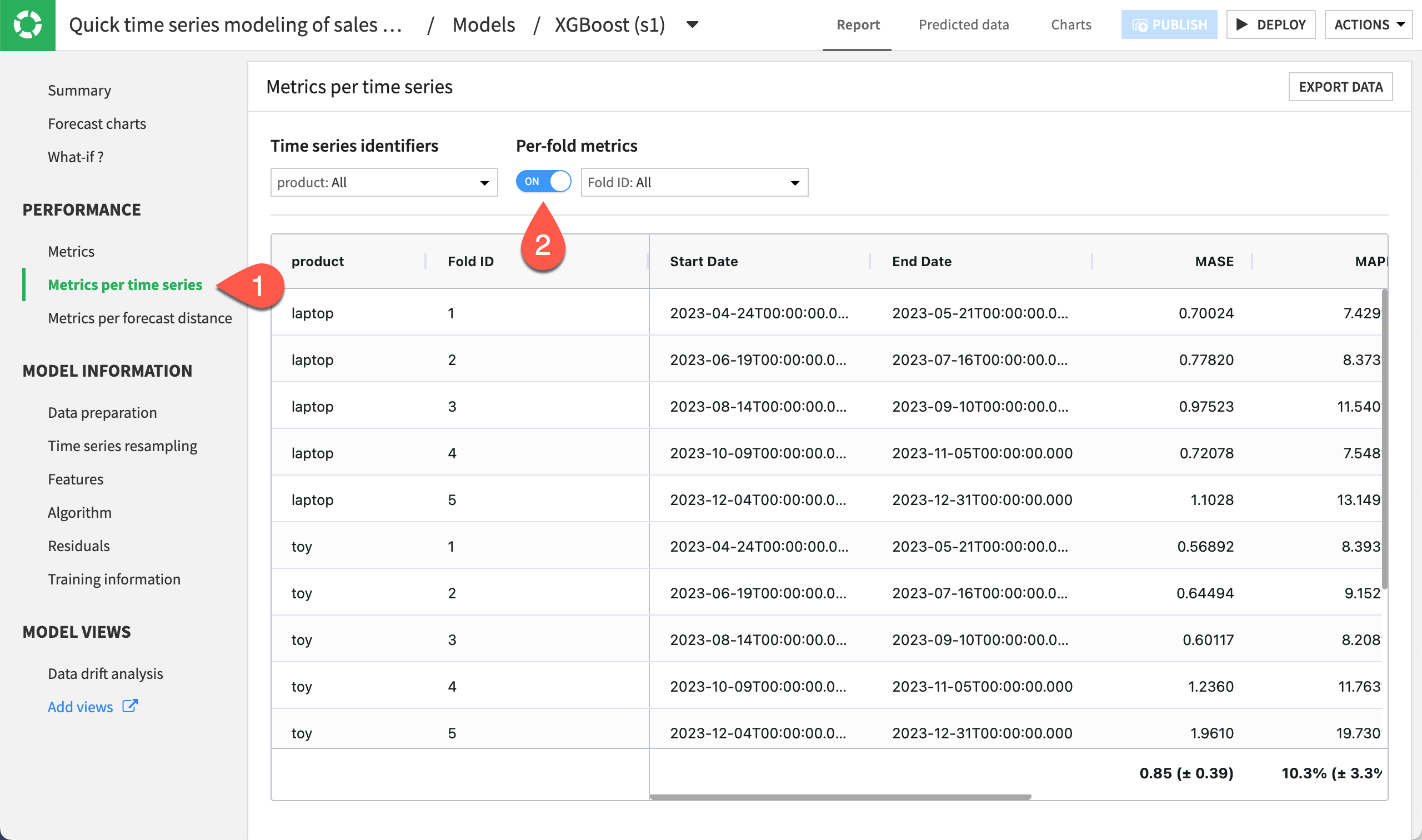
This way, you can see if any of the folds are under or overperforming relative to the others. This allows you to better control the performance of your model training and predictions.
View forecast charts#
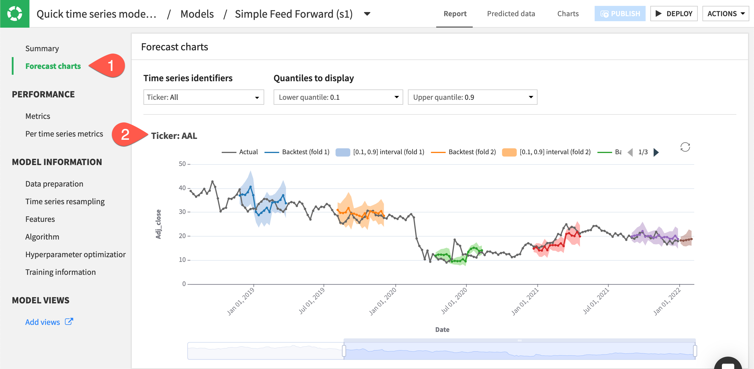
Look closer at this model’s forecast.
Still in the Report tab, navigate to the Forecast charts panel.
Inspect the predictions for each time series plot.
Note
The other panels of the model’s Report page show additional training details. For example, the Metrics tab in the Performance section displays the aggregated metrics for the overall dataset and its individual time series. The tabs in the Model Information section provide more details on resampling, features used to train the model, the algorithm details, etc.
Explore forecast scenarios with What if? analysis#
After training the forecasting model, use the What if? analysis interface to interactively explore how changes in input features would affect predictions. Any set of modifications you apply can be saved as a scenario, allowing you to revisit, compare, and iterate on different hypotheses without re-entering changes.
Create and explore the default scenario#
Let’s begin by creating the default scenario, which reflects the model forecast after the first training.
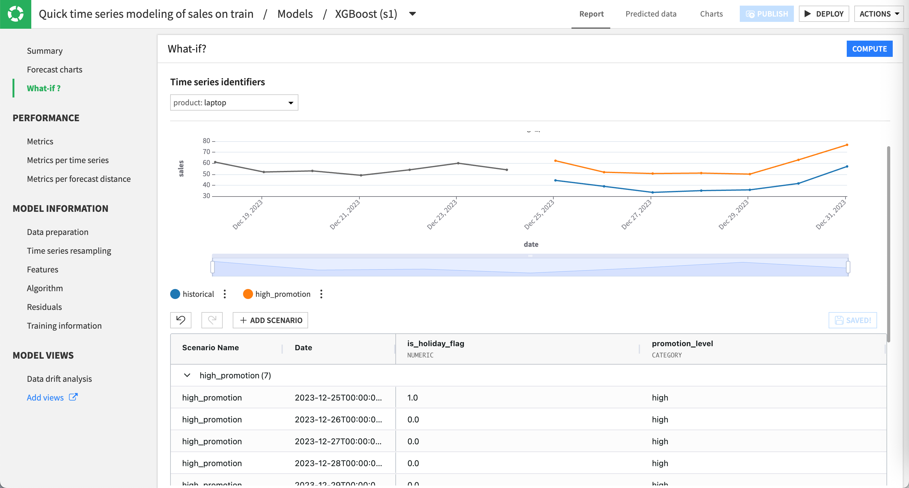
Still in the Report tab, navigate to the What-if? panel. This action automatically creates a default scenario for the selected product.
Click Compute to display the forecast on the top chart.
As you can see, the forecast extends from the end of the training data into the first horizon defined during model design. The editable grid includes the two input features used by the model (is_holiday_flag and promotion_level), allowing you to modify their values for the same horizon or future ones. You could edit any value in the grid of this default scenario to see how changes would impact the forecast. Yet, let’s experiment in another scenario to keep this one as a reference and compare them.
Note
By default, the interface displays the forecast for the laptop product. You can switch to toy or tshirt using the time series identifier selector.
Add a new scenario#
Now, you’ll create a scenario to explore how a higher promotion level affects the sales forecast. In this example, you’ll define a scenario that introduces a high promotion level for the
same horizon as the default scenario.
Click the + Add Scenario button.
Name the scenario
high_promotion.Keep the From 2023-12-25T00:00:00.000 (forecasting last horizon) selected.
Click Create Scenario.
In the grid, set the value of promotion_level to
highfor each line of the new scenario. Dataiku highlights modified cells in yellow.Note
You can do a bulk edit using the copy-paste functionality to fill in multiple cells with the same value. Enter
highin the first cell, then copy it and select the range of cells below to paste the value.Click Compute.
Review the updated chart. Dataiku displays the default scenario in blue and the new high_promotion scenario in orange.
Note
Any time, you can rename, delete or duplicate scenarios by clicking on More options (![]() ) next to the scenario name.
) next to the scenario name.
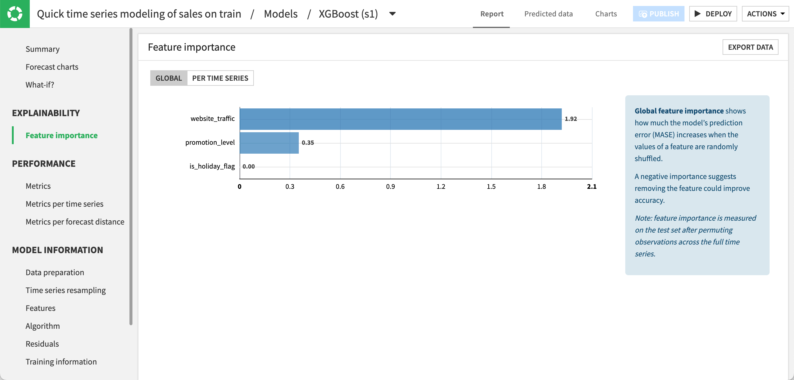
Explore feature importance#
You can analyze the importance of features used by the model to understand how each input variable contributes to the model’s forecasts. This can help you decide whether or not to retrain the model with features that contribute little relative to their acquisition or preparation cost.
Still in the Report tab, navigate to the Feature importance panel.
Under Global, click Compute Now to compute the feature importance across all time series. As you can see, website traffic is the feature that influences the predictions for the model the most, followed by the promotion level.
Under Per Time Series, click Compute Now to compute the feature importance separately for each time series. The relative importance of features may vary across products. Here, the website traffic has a stronger influence for toys and t-shirts than for laptops.
Deploy the model to the Flow#
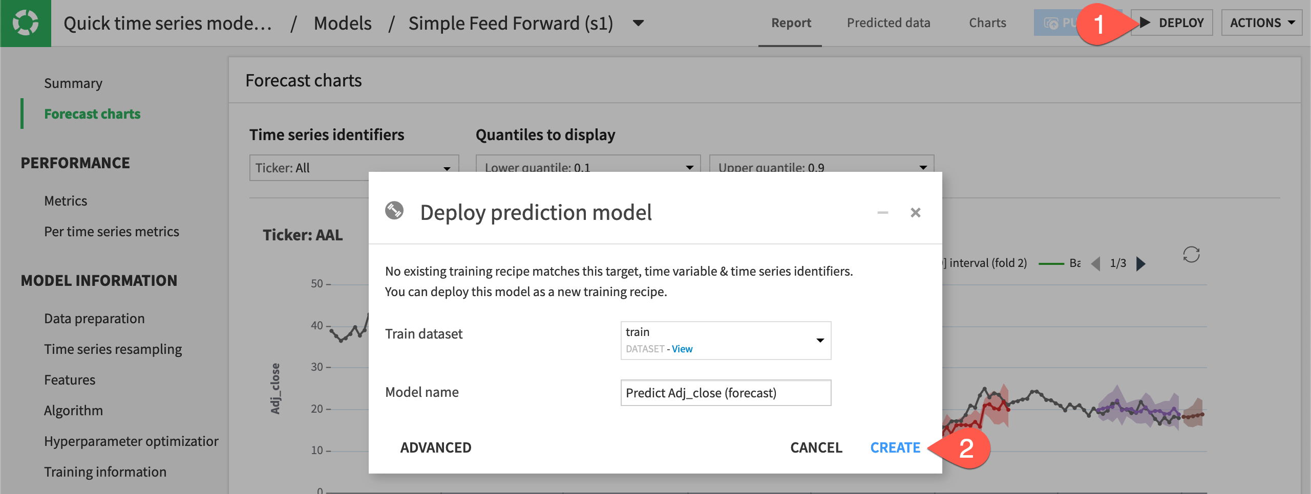
Once you finish inspecting the model and are satisfied with its performance, you can deploy the model to the Flow.
Click Deploy from the top right corner of the model page.
Click Create to deploy the Predict sales (forecast) model to the Flow.
Note
Like any other Dataiku visual ML model, you can deploy time series models in the Flow for batch scoring or as an API for real-time scoring.
Evaluate a forecasting model#
Next, you’ll evaluate the model’s performance on data not used during training. For this, you’ll use the Evaluate recipe.
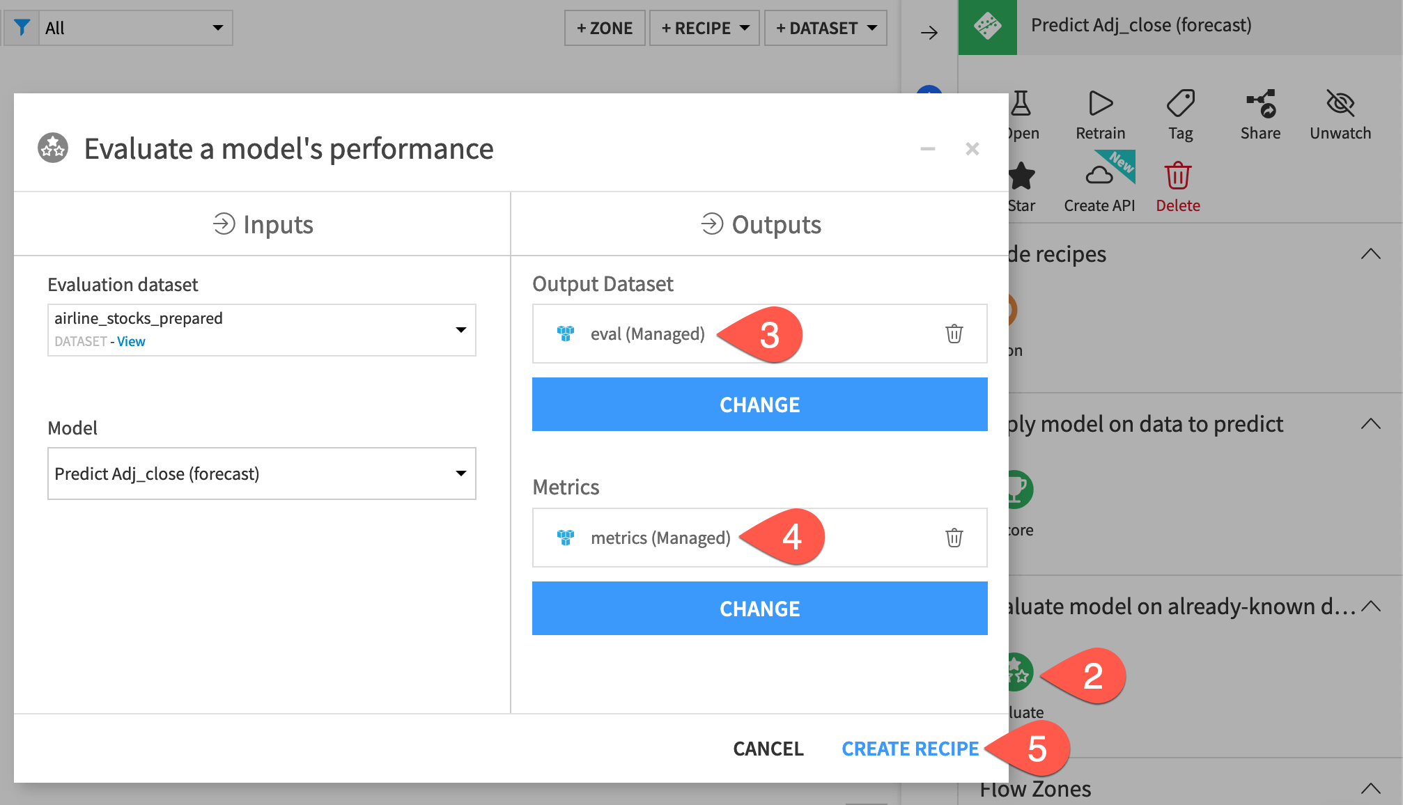
Create an Evaluate recipe#
To apply the Evaluate recipe to the time series model, you’ll use a validation set from the eval dataset as input. The validation set will include the time series values after January 1, 2024.
From the Flow, select both the eval dataset and Predict sales (forecast) model.
In the Actions panel on the right, select the Evaluate recipe.
Click Set to add an output dataset. Name it
eval_output, and click Create Dataset.Click Set to add metrics. Name it
eval_metrics, and click Create Dataset.Click Set to add an evaluation store. Name it
eval_store, and click Create Evaluation Store.Once you have inputs, outputs, and the evaluation store created, click Create Recipe.
Configure the Evaluate recipe#
On the recipe’s Settings page, Dataiku alerts as to how much past data is required according to the model’s specifications.
Note
If you used external features while training the model, Dataiku would require that the input data to the Evaluate recipe contain values for the external features. This requirement is also true when you use the Scoring recipe.
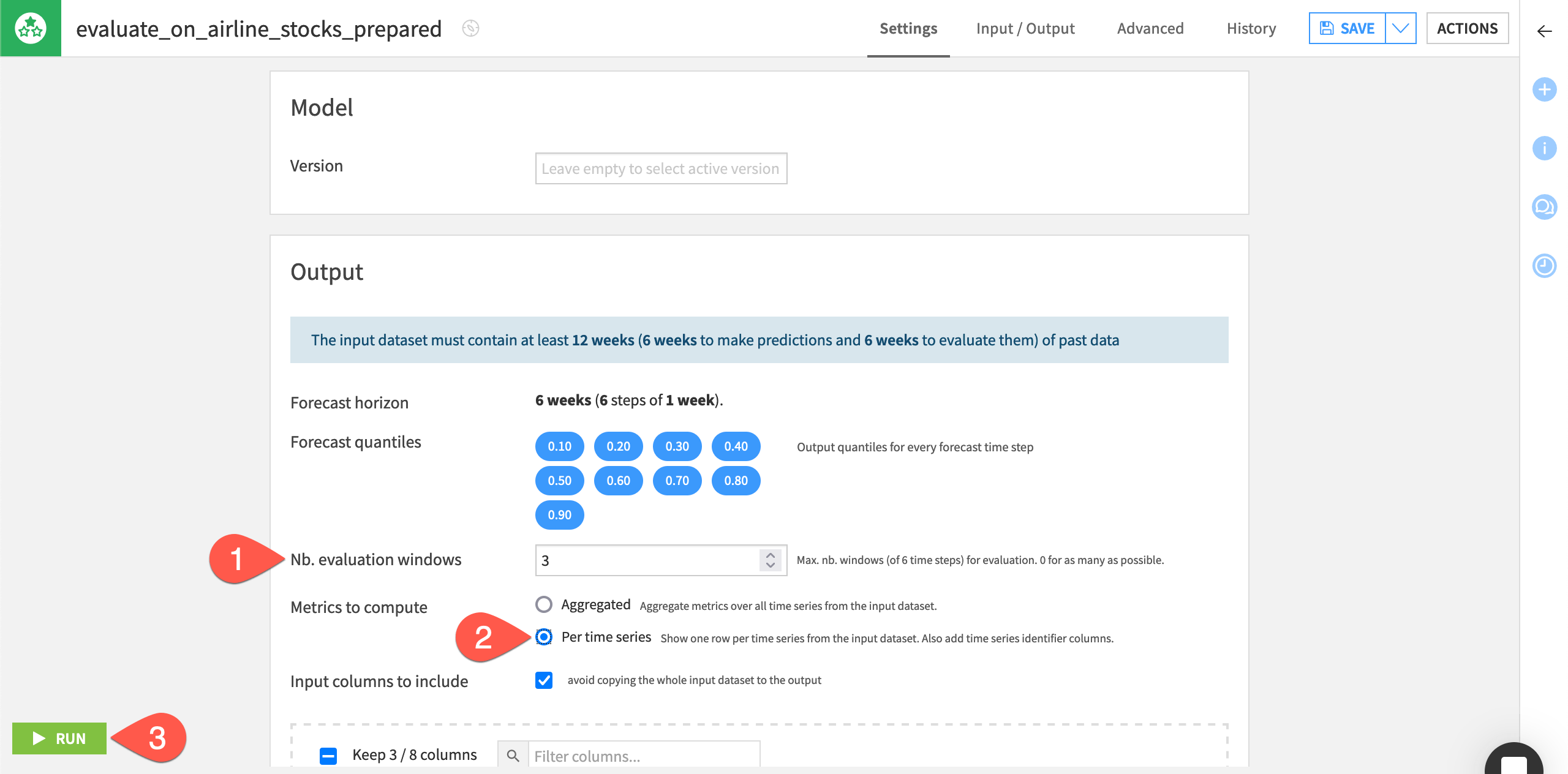
By default, the recipe uses a forecast horizon of six weeks (six steps in advance) since this was the model’s setting during training. Dataiku also outputs forecast values at different quantiles (the same ones used during training).
Specify the remaining settings for the recipe as follows:
On the Settings tab of the recipe, leave the Nb. evaluation time steps values as
0to use the maximum number of evaluation windows.Instead of aggregated metrics, select the option to compute metrics Per time series for Dataiku to show one row of metrics per time series.
Click Run to execute the recipe.
Explore the evaluation results#
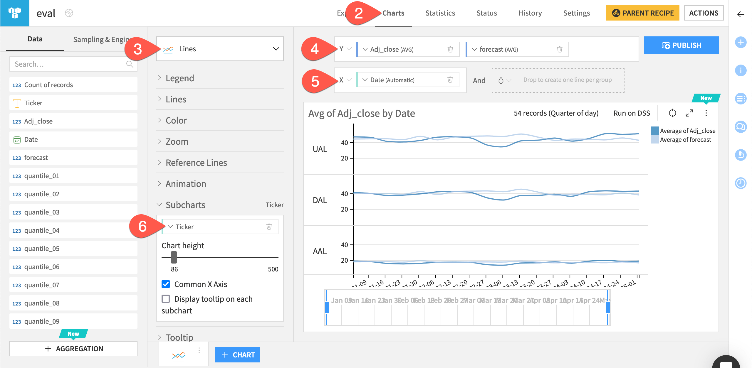
In the eval dataset, you can view the actual values of the sales prices and the forecasts. You can also create line charts on the dataset to compare the forecasts to the actual time series values.
Open the eval_output dataset, and explore the added forecast column.
Navigate to the Charts tab.
From the chart picker, select a Lines plot.
Drag sales and forecast to the Y-axis field.
Drag date to the X-axis field.
Click date and select Week as Date range to have a weekly view of the chart.
Drag product to the Subcharts option to the left of the chart. Adjust the chart height as needed.
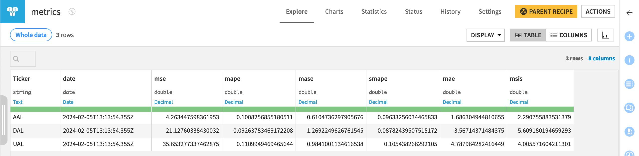
In addition to the forecast values, you can also examine the associated metrics.
Return to the Flow.
Open the eval_metrics dataset to see one row of metrics per time series, per run of the Evaluate recipe.
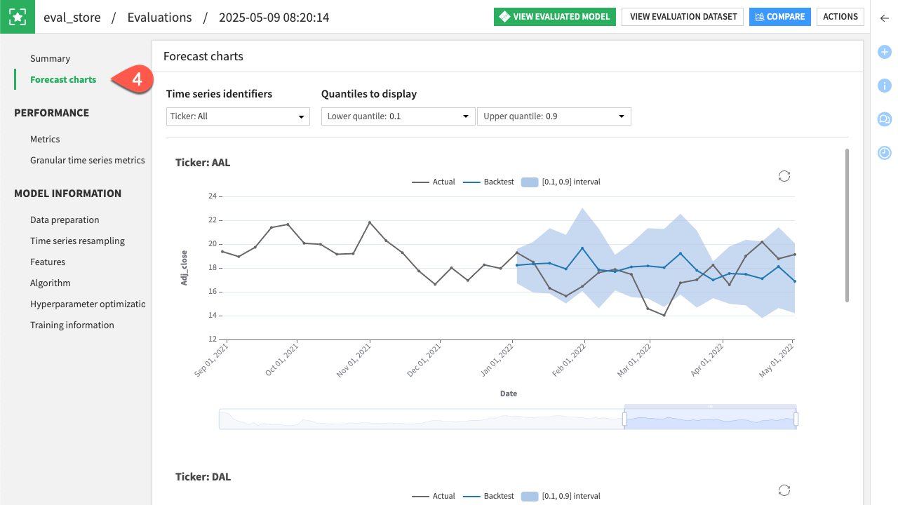
For more in-depth evaluation monitoring, you can check the evaluation store created before.
Return to the Flow.
Open the eval_store evaluation store.
Under Model Evaluation, click Open on the latest evaluation.
Note
Notice that on this page you have an overview of all the evaluations of this model with a list of relevant statistics.
Navigate to the Forecast charts tab to visually explore the different forecasts the model has made for each product.
Score a forecasting model#
Finally, you’ll apply a Score recipe to the model to predict future values of the time series.
Create a Score recipe#
To apply the Score recipe to the time series model, you’ll use the scoring dataset as input. The Score recipe will use this input with the trained model to forecast future values of the time series (for dates after January 1, 2025).
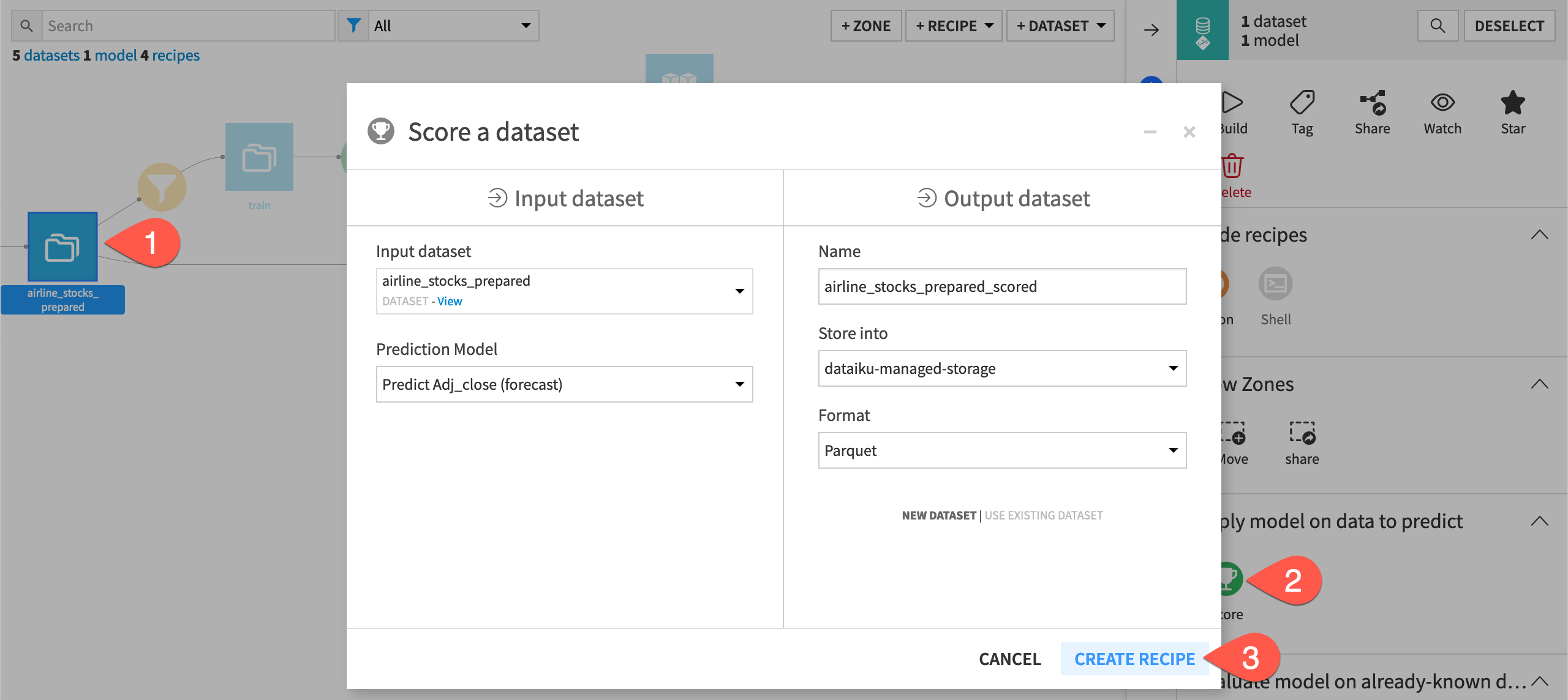
From the Flow, select both the scoring dataset and Predict sales (forecast) model.
In the Actions panel on the right, select the Score recipe.
Click Create Recipe.
Configure the Score recipe#
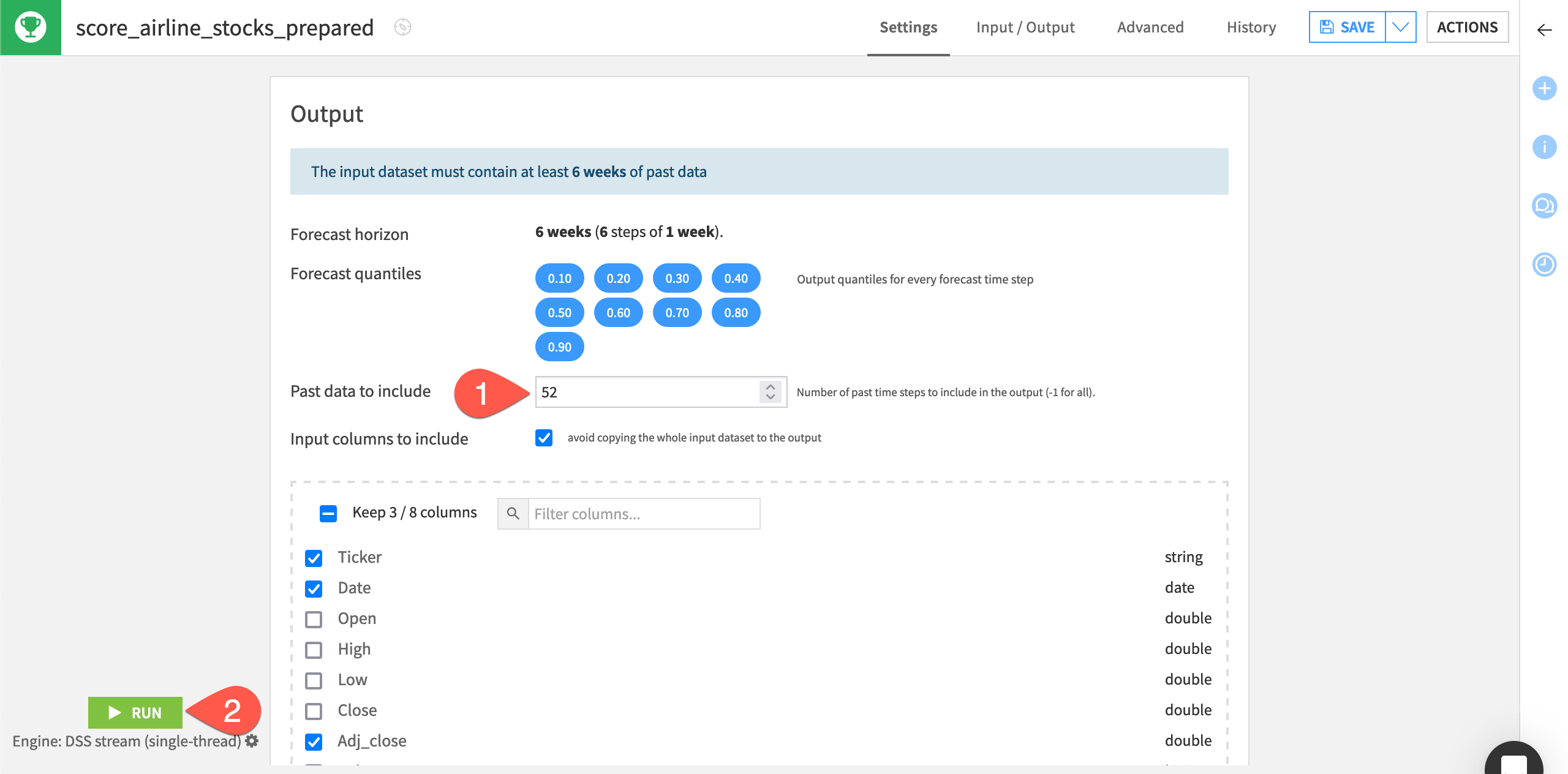
Similar to the Evaluate recipe, Dataiku alerts you as to how much past data must be found in the input dataset.
By default, the recipe uses a forecast horizon of 7 days since this was the model’s setting during training. Dataiku also outputs forecast values at different quantiles (the same ones used during training).
Leave the forecast length by default to
7.Set the Past data to include at
28days.Click Run to execute the recipe.
Inspect the scored data#
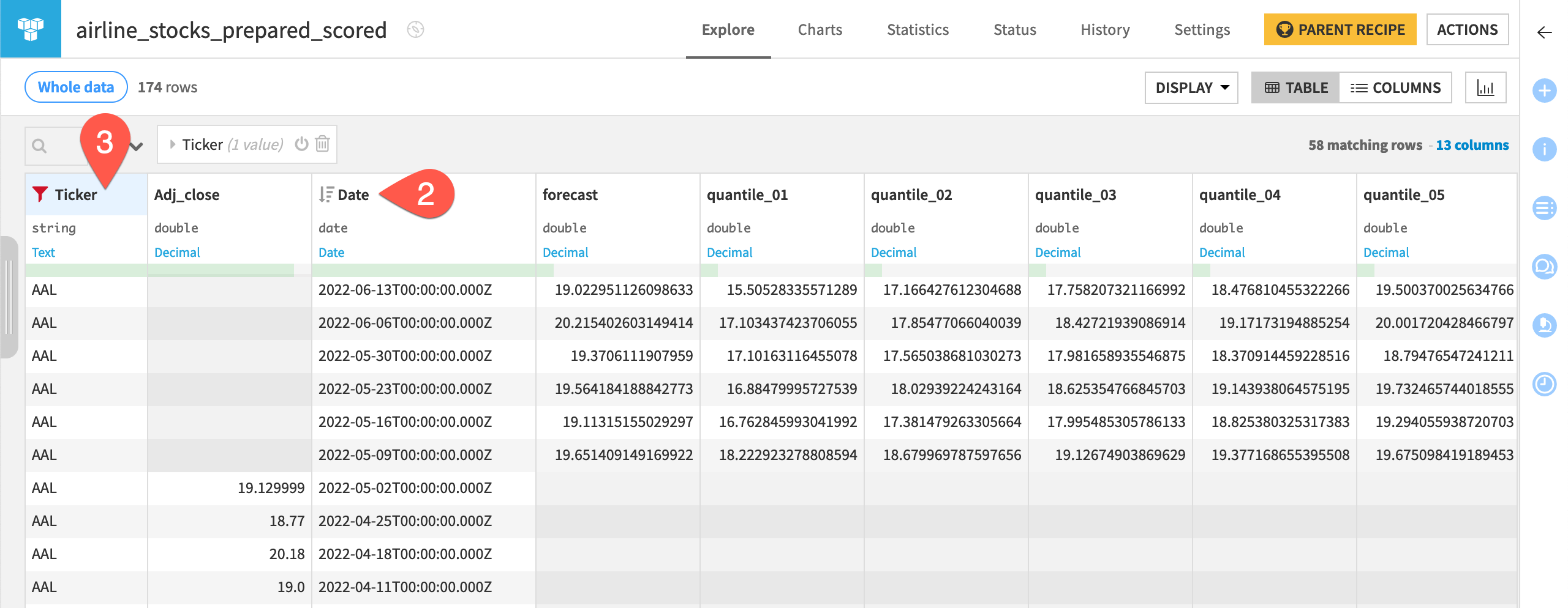
The recipe forecast values of the sales alongside the quantiles for the next seven days for each of the product.
When the Score recipe finishes, open the scoring_scored dataset.
Click on the date column header, select Sort, and then click the icon to sort in descending order to see the forecasted values at the top of the dataset.
Click on the product column header, select Filter, and then select a series such as laptop to view an individual series.
Note
The reference documentation provides more information on using the Score recipe with a time series model.
Next steps#
Congratulations! You’ve taken your first steps toward forecasting time series data using Dataiku’s visual ML interface.
See also
Learn more in the reference documentation on Time Series Forecasting.
You can also explore an example project demonstrating various visual time series forecasting techniques in the Dataiku Gallery.