Hands-On Tutorial: Window Recipe (Deep Dive)

For all the potential that they offer, window functions can be tricky to code successfully. The visual Window recipe in Dataiku, however, allows you to take advantage of these powerful features without coding.

Let’s Get Started!

The previous hands-on tutorial provided an introduction to the Window recipe, but mastering all of the possible variations of this recipe can be challenging.

Accordingly, this tutorial includes five more examples using the same credit card transactions use case–each of which demonstrates a different aspect:

• basic grouped aggregation,

• ranking,

• a cumulative sum,

• a moving average, and

• a lagged calculation.

Note

We encourage completing this tutorial to strengthen your ability to use the Window recipe. However, future lessons do not depend on the specific work done here, and so for that reason, it is optional.

Advanced Designer Prerequisites

This lesson assumes that you have basic knowledge of working with Dataiku DSS datasets and recipes.

Note

If not already on the Advanced Designer learning path, completing the Core Designer Certificate is recommended.

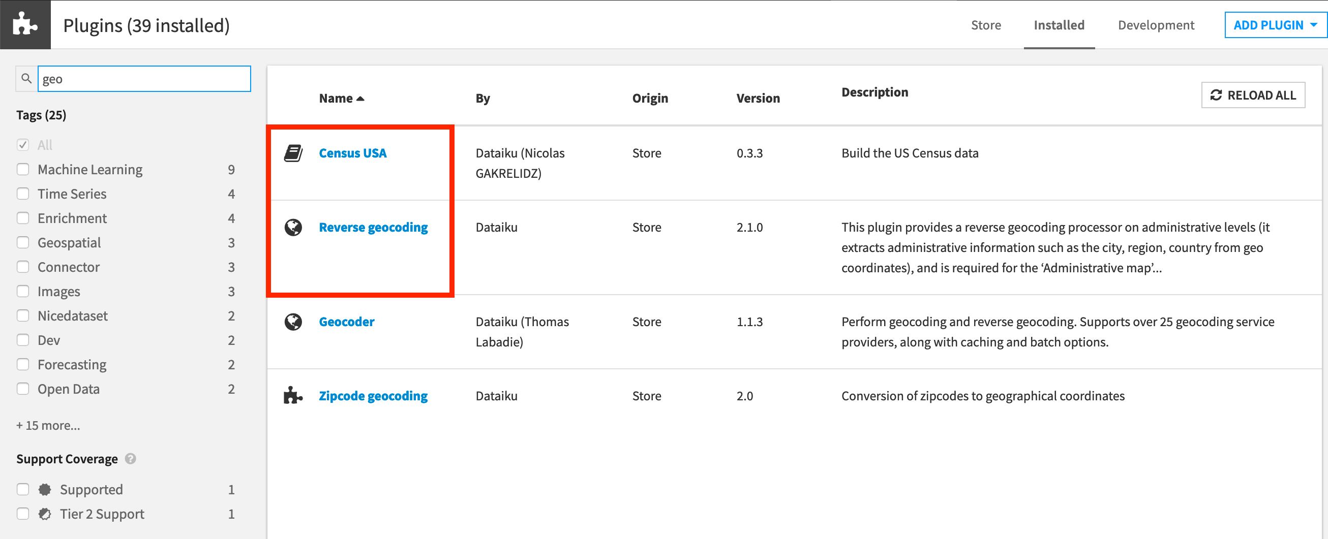
To complete the Advanced Designer learning path, you’ll need access to an instance of Dataiku DSS (version 8.0 or above) with the following plugins installed:

• Census USA (minimum version 0.3)

• Reverse geocoding

These plugins are available through the Dataiku Plugin store, and you can find the instructions for installing plugins in the reference documentation. To check whether the plugin is already installed on your instance, go to the Installed tab in the Plugin Store to see a list of all installed plugins.

Note

If your goal is to complete only the tutorials in Visual Recipes 102, the Census USA plugin is not required.

In order to get the most out of this lesson, we recommend completing the following lessons beforehand:

• Concept: Window Recipe

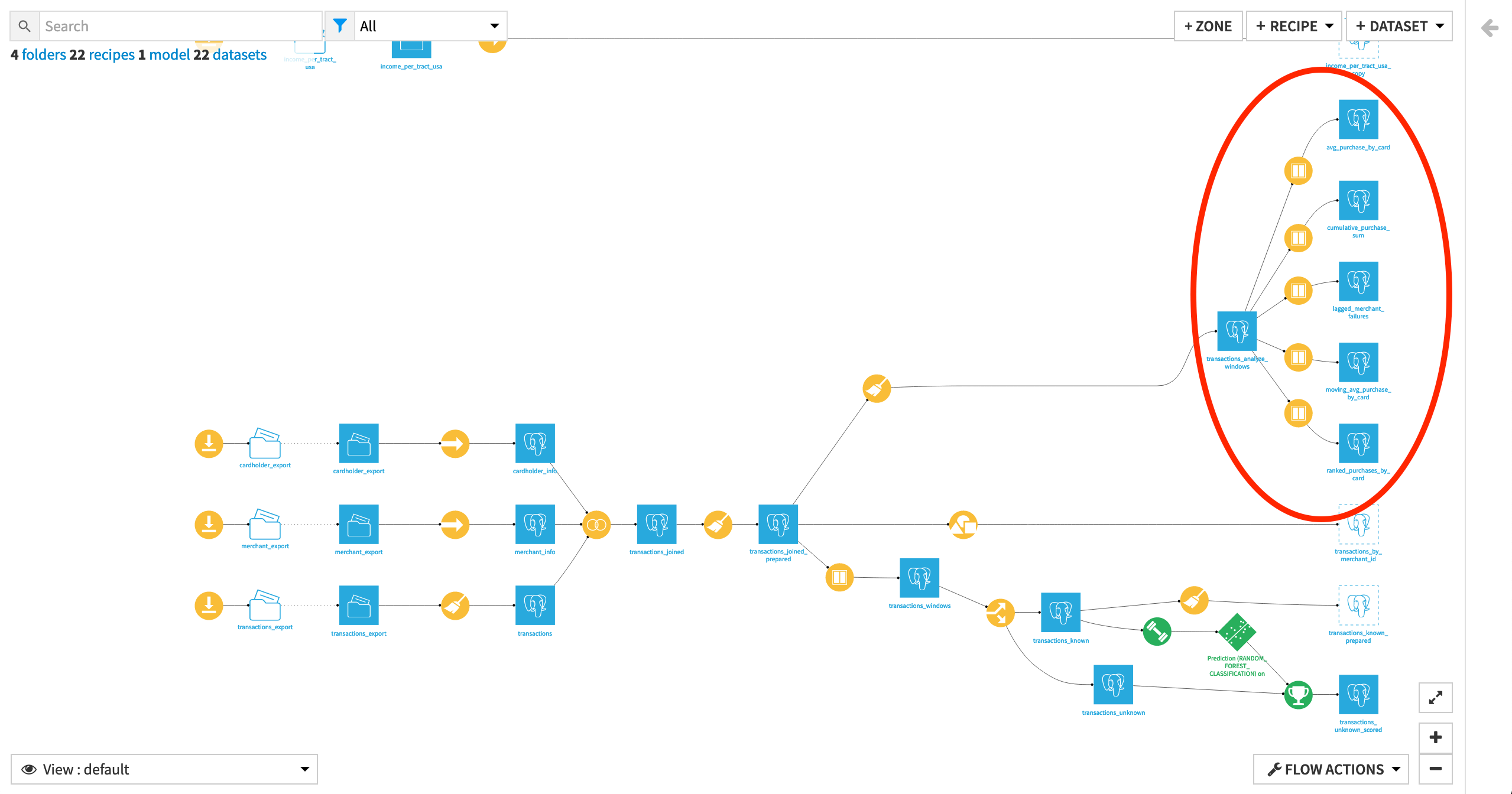
Workflow Overview

In this tutorial, we’ll be demonstrating five Window recipes with different window definitions to answer various kinds of questions.

Create Your Project

• Click +New Project > DSS Tutorials > Advanced Designer > Window Recipe (Tutorial).

Note

If you’ve already completed the other Window recipe hands-on tutorial, you can use the same project.

Note

You can also download the starter project from this website and import it as a zip file.

Change Dataset Connections (Optional)

Aside from the input datasets, all of the others are empty managed filesystem datasets.

You are welcome to leave the storage connection of these datasets in place, but you can also use another storage system depending on the infrastructure available to you.

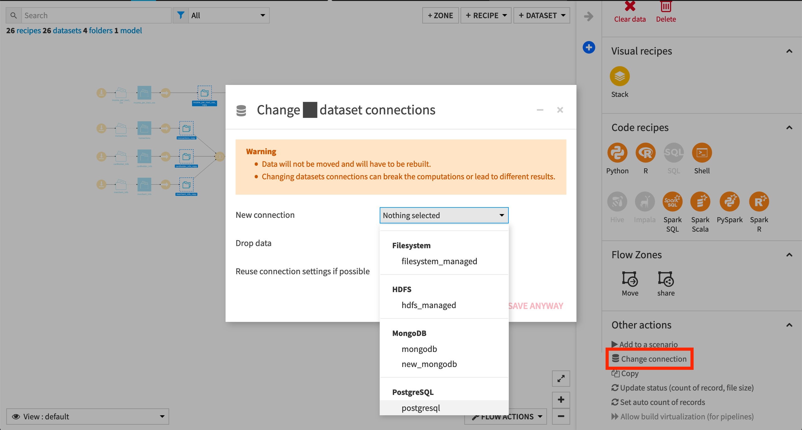
To use another connection, such as a SQL database, follow these steps:

• Select the empty datasets from the Flow. (On a Mac, hold Shift to select multiple datasets).

• Click Change connection in the “Other actions” section of the Actions sidebar.

• Use the dropdown menu to select the new connection.

• Click Save.

Note

For a dataset that is already built, changing to a new connection clears the dataset so that it would need to be rebuilt.

Note

Another way to select datasets is from the Datasets page (G+D). There are also programmatic ways of doing operations like this that you’ll learn about in the Developer learning path.

The screenshots below demonstrate using a PostgreSQL database.

• Whether starting from an existing or fresh project, ensure that the dataset transactions_analyze_windows is built. It is the same as the transactions_joined_prepared dataset, but with a smaller selection of columns for convenience.

See Build Details Here if Necessary

• From the Flow, select the end dataset required for this tutorial: transactions_analyze_windows

• Choose Build from the Actions sidebar.

• Choose Recursive > Smart reconstruction.

• Click Build to start the job, or click Preview to view the suggested job.

• If previewing, in the Jobs tab, you can see all the activities that Dataiku will perform.

• Click Run, and observe how Dataiku progresses through the list of activities.

Basic Grouped Aggregation with the Window Recipe

The Window recipe has many similarities with the Group recipe.

For example, we could find out the average purchase amount of every card_id with a simple Group recipe. However, the output would dataset would be reduced to the group key and the aggregated columns. The structure of the original dataset would be lost, which would make it more difficult to use those aggregations as features.

• With the transactions_analyze_windows dataset selected, choose Actions > Window in the right panel to create a new Window recipe.

• Name the output dataset avg_purchase_by_card.

Warning

When working with file-based datasets and using the default DSS engine to run recipes, Order Columns and Window Frame should be activated in order for the Window recipe to output the same results as when working with most SQL-based datasets. For this reason, some of the examples below require slightly different Window definitions.

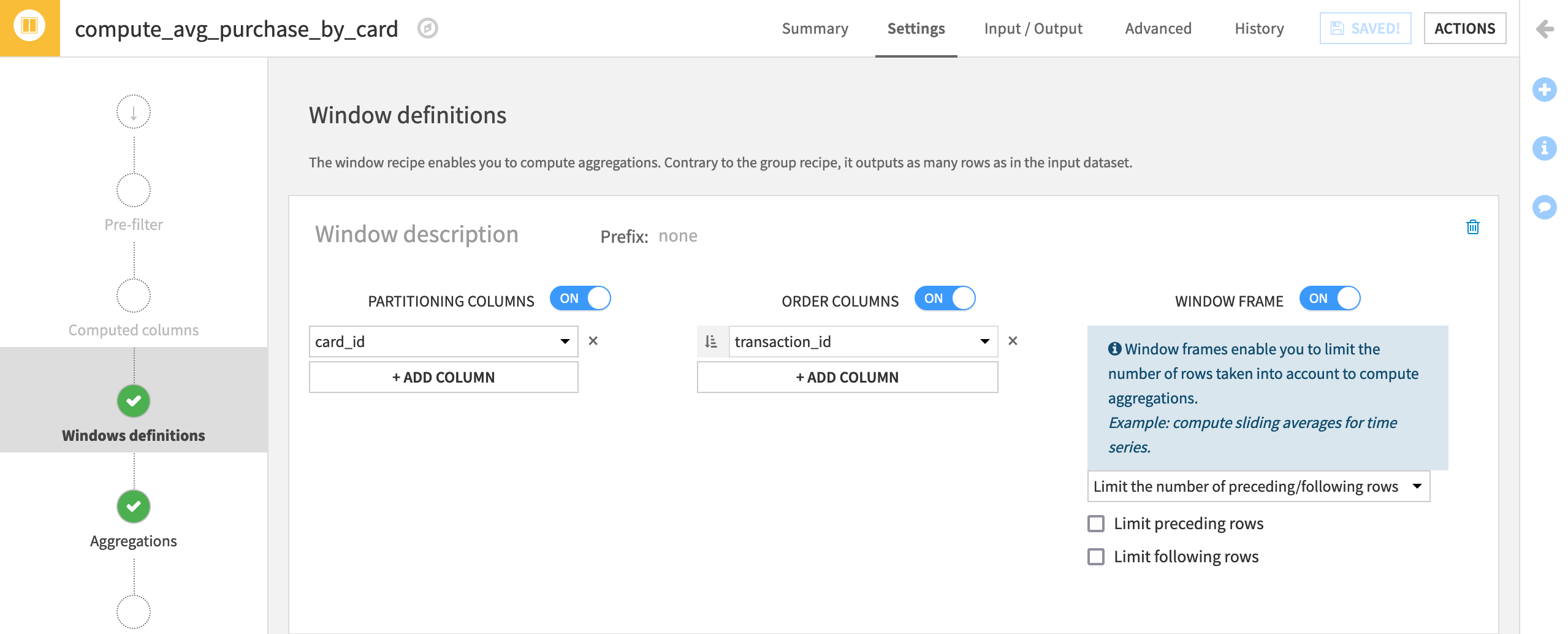
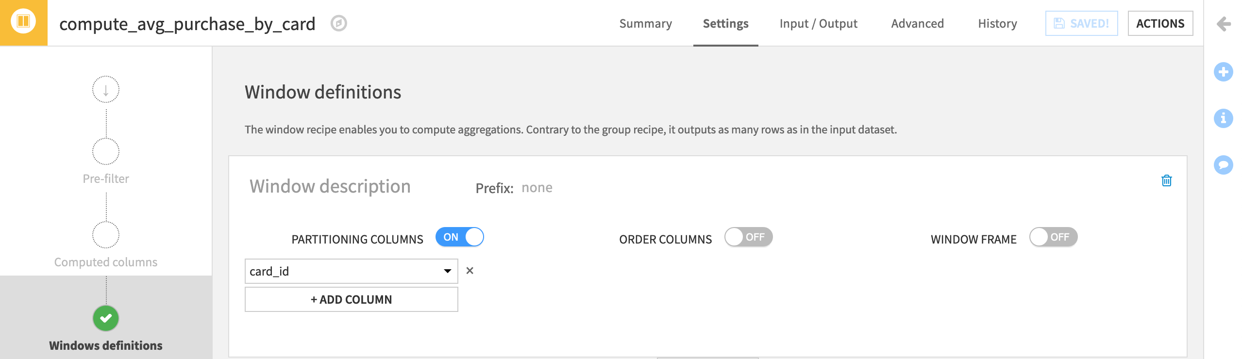
Window definition step for file-based datasets

• On the Window definition step, turn on Partitioning Columns, and choose card_id.

• Turn on Order Columns (the unique identifier transaction_id should already be selected).

• Turn on Window Frame, but do not limit any rows.

Window definition step for SQL-based datasets

• On the Window definition step, turn on Partitioning Columns, and choose card_id.

Note

When we partition by columns in the Window recipe, we are not creating separate datasets. We are partitioning the dataset by the selected column(s), in our case, by card_id. Dataiku DSS will create partitions, or groups, for each credit card, while keeping the data as a single dataset.

• Once the window is defined, on the Aggregations step, add the Avg of purchase_amount.

• Run the recipe, updating the schema.

In the output dataset, filter for a single card_id to more easily see that the new purchase_amount_avg column is the same for every unique card_id.

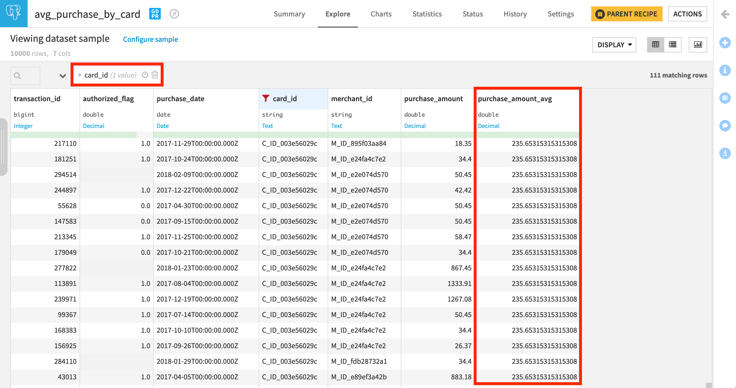
We could have calculated the same average purchase results with a Group recipe. However, in this format, it would be easier to compute, for example, the difference between the average amount for a given card and the amount of an individual transaction, to get a notion of whether any particular transaction may be unusually high for this card.

Compute Ranks

The example above made use of a partitioning column, but not an order column. An order column makes possible many new kinds of aggregations.

For example, we might also be interested in questions like, “What is the most expensive purchase for every card_id?” To answer this question, we’ll use a partitioning column, an order column, a rank aggregation, and finally a post-filter step.

• With the transactions_analyze_windows dataset selected, choose Actions > Window to create a new Window recipe.

• Name the output dataset ranked_purchases_by_card.

Let’s start by defining the correct window.

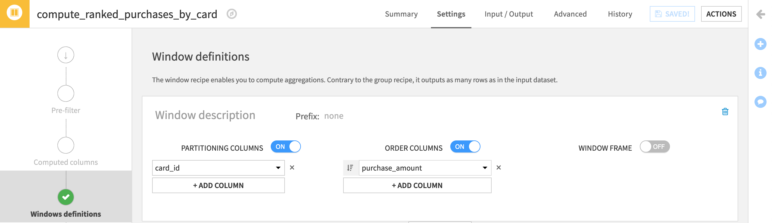
• Just as in the above example, we are still interested in information per card_id, and so choose this as the Partitioning Column.

• Turn on Order Columns. We want the most expensive purchase per card_id to have a rank of 1, and so we want to order rows by purchase_amount in descending order .

Then set the window frame depending on the connection in your project:

Window frame for file-based datasets

• Turn on the Window Frame, but do not limit any rows.

Window frame for SQL-based datasets

• Leave the Window Frame turned off.

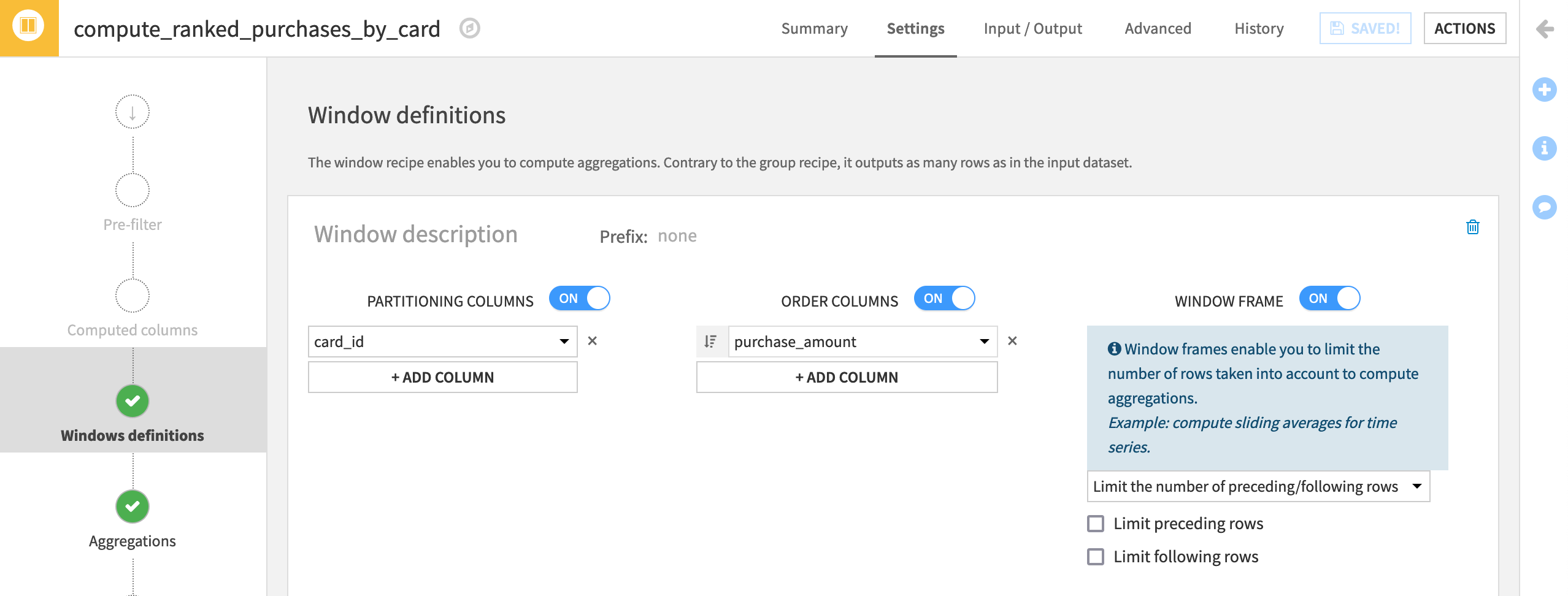
• On the Window aggregations step, we only want to focus on one aggregation. Enable Rank, and then run the recipe.

Note

Rank is the “index” of the current row within its window. In other words, since we have a window partitioned by card_id, and ordered by decreasing purchase_amount, the most expensive transaction of each item_category will have rank=1, the second most expensive transaction of each group will have rank=2, and so on.

In the output dataset, once again filter for a single card_id to more easily notice how ranks are assigned according to the most expensive purchase per card_id.

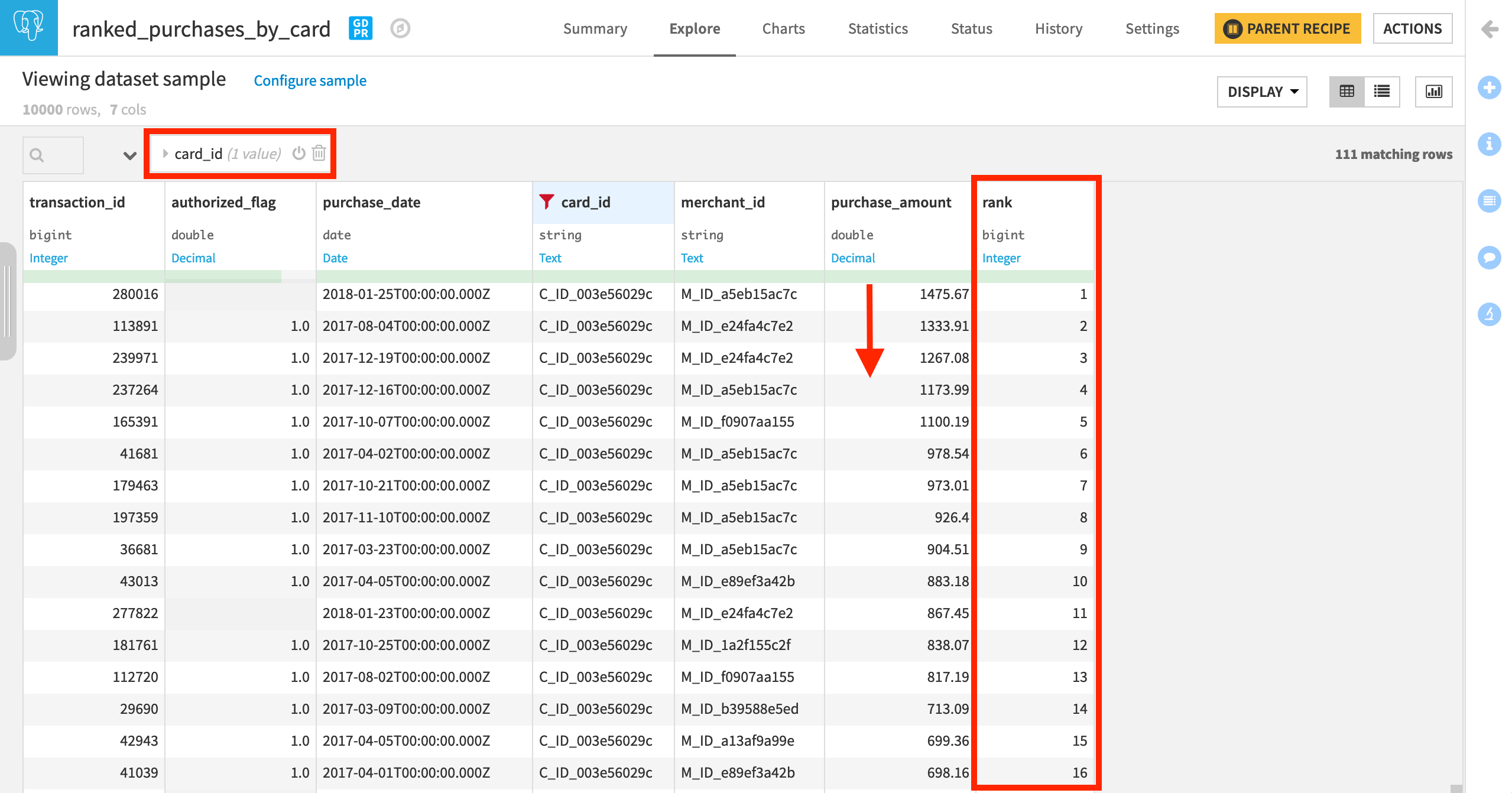
Tip

To find the most expensive purchase per card, return to the parent recipe, and apply a post-filter of rank == 1.

Compute Cumulative Sums

None of the previous examples required actually limiting the window frame. Calculating a cumulative sum, however, does.

Imagine we’d like to know the proportion of the total purchase amounts made over time. In other words, we want to compute the cumulative distribution of the summed purchase amount. We’re no longer interested in partitioning by card_id; we want global information.

• With the transactions_analyze_windows dataset selected, choose Actions > Window to create a new Window recipe.

• Name the output dataset cumulative_purchase_sum.

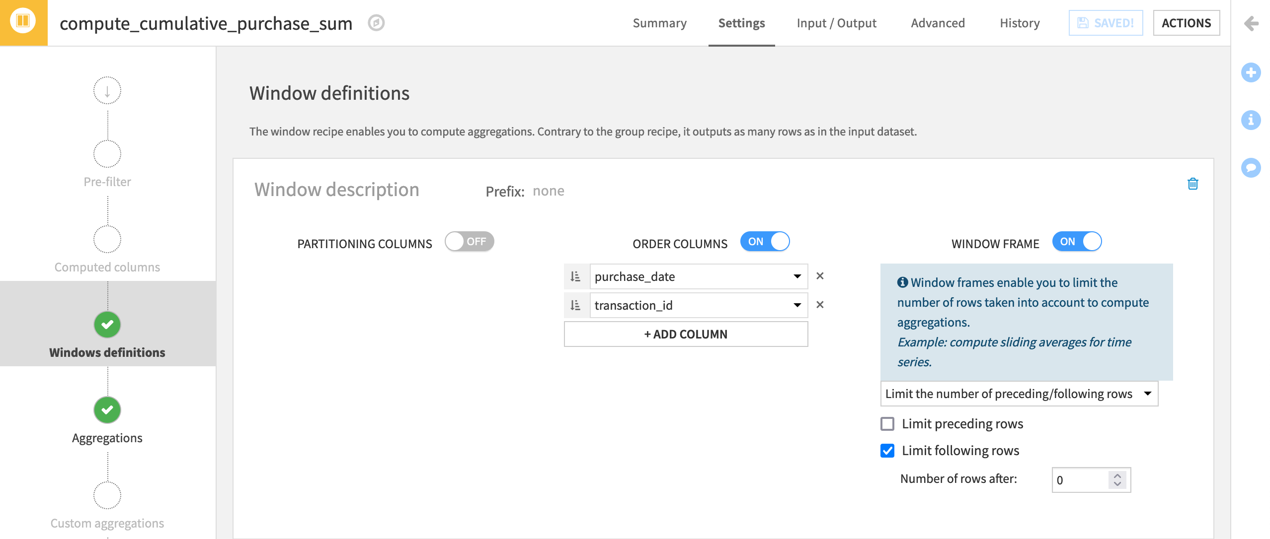
In the Window definition step, we’ll now use an order column and window frame, but not a partitioning column.

• Leave Partitioning Columns off.

• Under Order Columns, select to order by purchase_date, and ensure that dates are sorted in ascending (chronological) order .

• Add transaction_id as a second Order column.

• Activate the Window Frame, and limit the number of following rows to 0.

Note

transaction_id is included as a second order column because purchase_date on its own does not guarantee a unique order (we have many purchases on the same day), and we are defining a window frame based on the number of preceding/following rows.

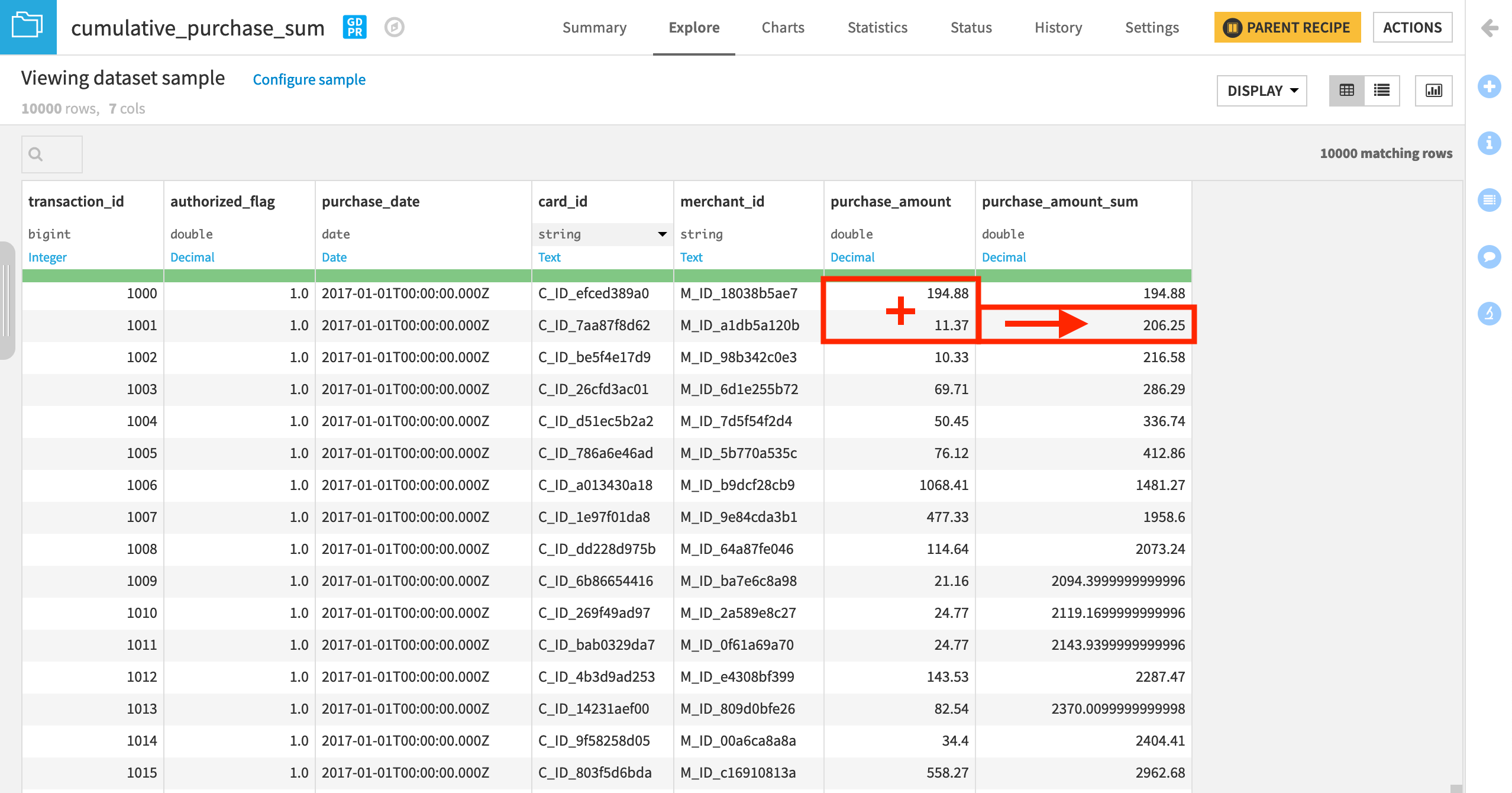
• On the Aggregations step, check the Sum box for purchase_amount.

• Then Run the recipe.

Since the window is ordered by purchase date and framed so as to not take into account following rows, this will compute the sum of the purchase amount of all previous transactions, plus the current one, for each transaction.

Visualize the Cumulative Sum (Optional)

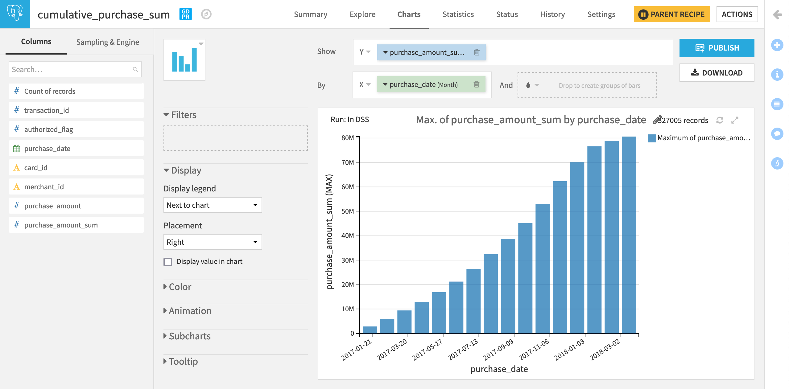
Let’s create a chart to visualize the cumulative sum.

• Navigate to the Charts tab of cumulative_purchase_sum.

• Drag purchase_amount_sum to the Y-axis and purchase_date as the X-axis.

• Change the Y-axis aggregation to MAX.

• Change the date range aggregation to “Month”.

To get the chart we want though, we’ll need to adjust the sample.

• Go to Sampling & Engine on the left panel

• Un-select Use same sample as Explore, and instead choose No sampling (whole data).

• Then save and refresh the sample.

Since we have ordered the window by purchase date, and there are multiple transactions for each date, the purchase_amount_sum value will increase with each new transaction. By selecting MAX as the aggregation, we look at the evolution in the cumulative sum of all purchase amounts at the end of each period.

Compute Moving Averages

Now we’re finally ready to see a partitioning column, an order column, and a window frame all working together at once.

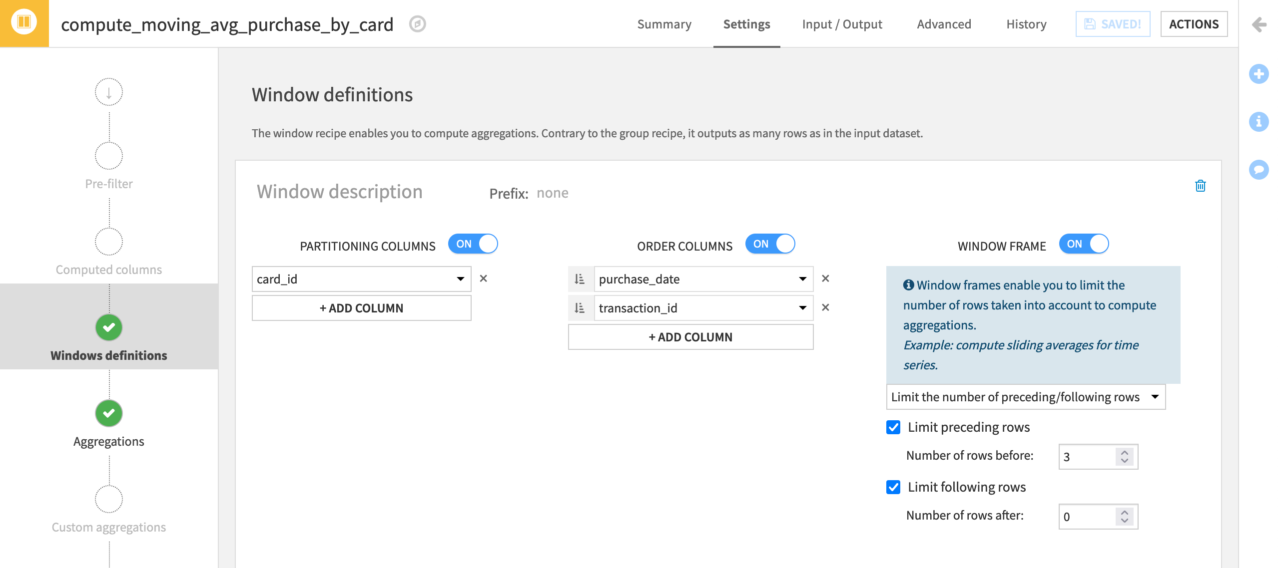
Instead of a single average purchase per card like in the first example, let’s create a moving average of the three most recent purchases on a given card (in addition to the present purchase). To do so, we’ll adjust the window frame setting to limit the window to the three preceding rows.

• With the transactions_analyze_windows dataset selected, choose Actions > Window to create a new Window recipe.

• Name the output dataset moving_avg_purchase_by_card.

Once you have created the recipe:

• Set card_id as the Partitioning Column.

• Just like for the cumulative sum, set purchase_date and transaction_id in ascending order as the Order Column.

• Activate the Window Frame, and limit the preceding rows to 3 (to include the three prior purchases) and the following rows to 0 (which includes the present row in the window frame).

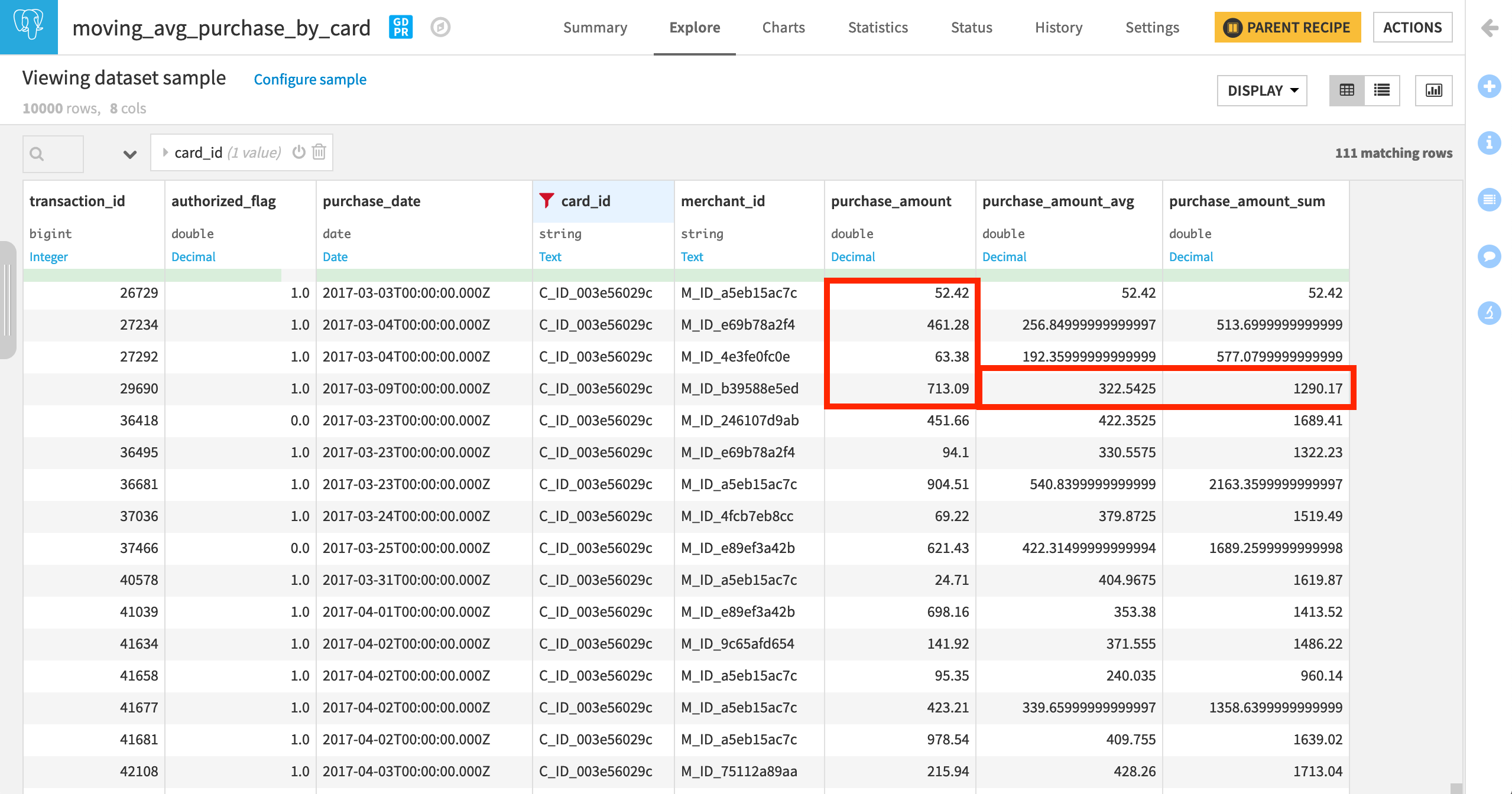
• On the Aggregations step, check the Avg and Sum (for easier verification) box for purchase_amount.

• Then Run the recipe.

In the output dataset, filter for a specific card_id to observe how card_purchase_amount_avg and card_purchase_amount_sum change along the window frame.

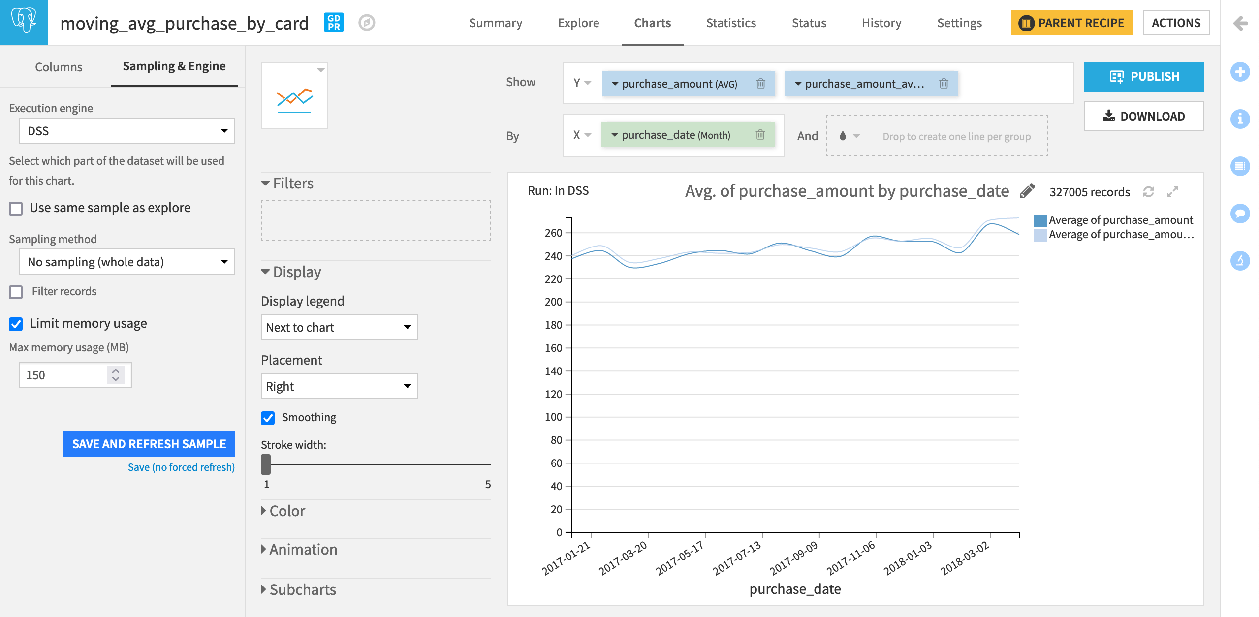
Visualize the Moving Average (Optional)

For the output dataset, we can chart the moving average along with the monthly average.

• In the Charts tab of the moving_avg_purchase_by_card dataset, choose Lines as the chart type.

• Drag purchase_amount and purchase_amount_avg to the Y-axis. (The aggregation should already be set to AVG).

• Drag purchase_date to the X-axis.

• Change the date range from Automatic to Month.

• Once again, adjust the sample to include the entire dataset.

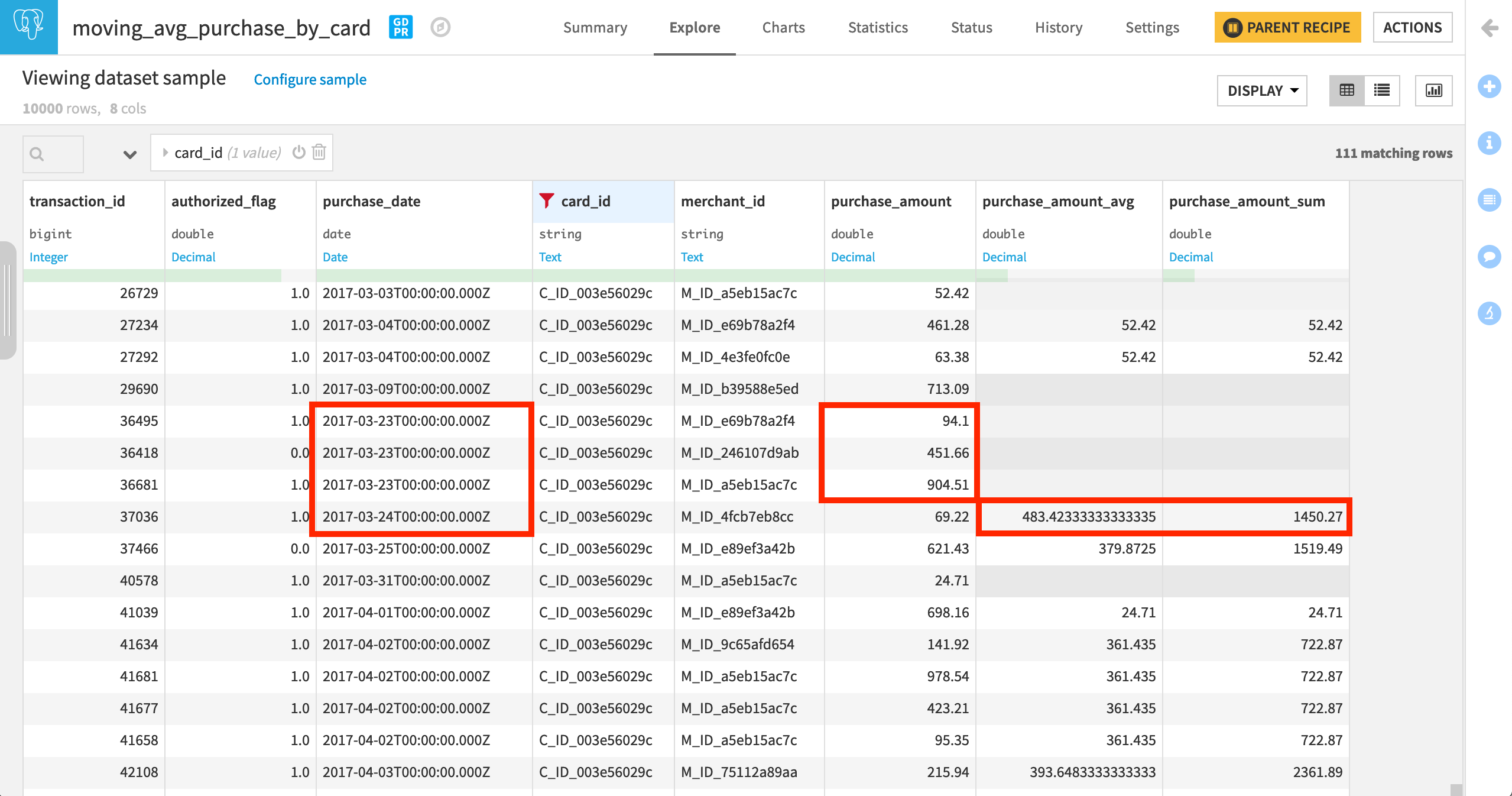
Limit the Window Frame on a Value Range of the Order Column

Instead of finding the average and sum of the three most recent purchases for every card, we might instead want to know about the sum and average of any number of purchases in the past three days on that card.

We can find this answer with a slight adjustment to the window frame.

• Return to the Window definition step of the recipe that computes moving_avg_purchase_by_card.

• Remove transaction_id as the second order column.

• Change the Window Frame setting to Limit window on a value range of the order column.

• Set the lower bound to 3 and the upper bound this time to -1 days (This will exclude the present row).

• Run the recipe again.

When filtering the output dataset for a single card_id, it’s possible to see the difference between these two window frames. For any card, there is no guarantee of a purchase every day, and so, the three previous rows and the three most recent days are not necessarily the same.

Note

When working with an irregular time series like this one, you might resample the data so no dates in the series are missing. This kind of operation can most easily be done with the Time Series Preparation Plugin, which you can learn about in this Academy course.

Compute Lag

One final example to introduce the very handy Lag and LagDiff aggregations!

Perhaps we are interested in whether certain merchants attract more fraud. We might want to investigate questions like, for any failed transaction:

• How many days have passed since a merchant’s last transaction failed authorization?

• How many failed transactions has a merchant had in the prior three days?

The Lag and LagDiff aggregations can help answer these kinds of questions.

• From the transactions_analyze_windows dataset, create a new Window recipe.

• Name the output lagged_merchant_failures.

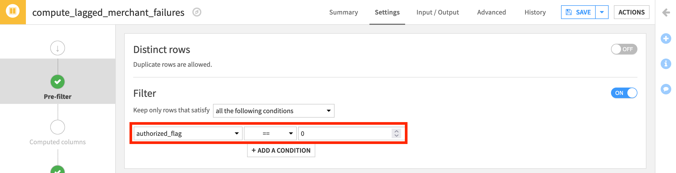
For the questions above, we are only interested in transactions that have failed authorization so we’ll need to use a pre-filter.

• On the Pre-filter step, activate the filter, and add the condition to keep only rows where authorized_flag == 0.

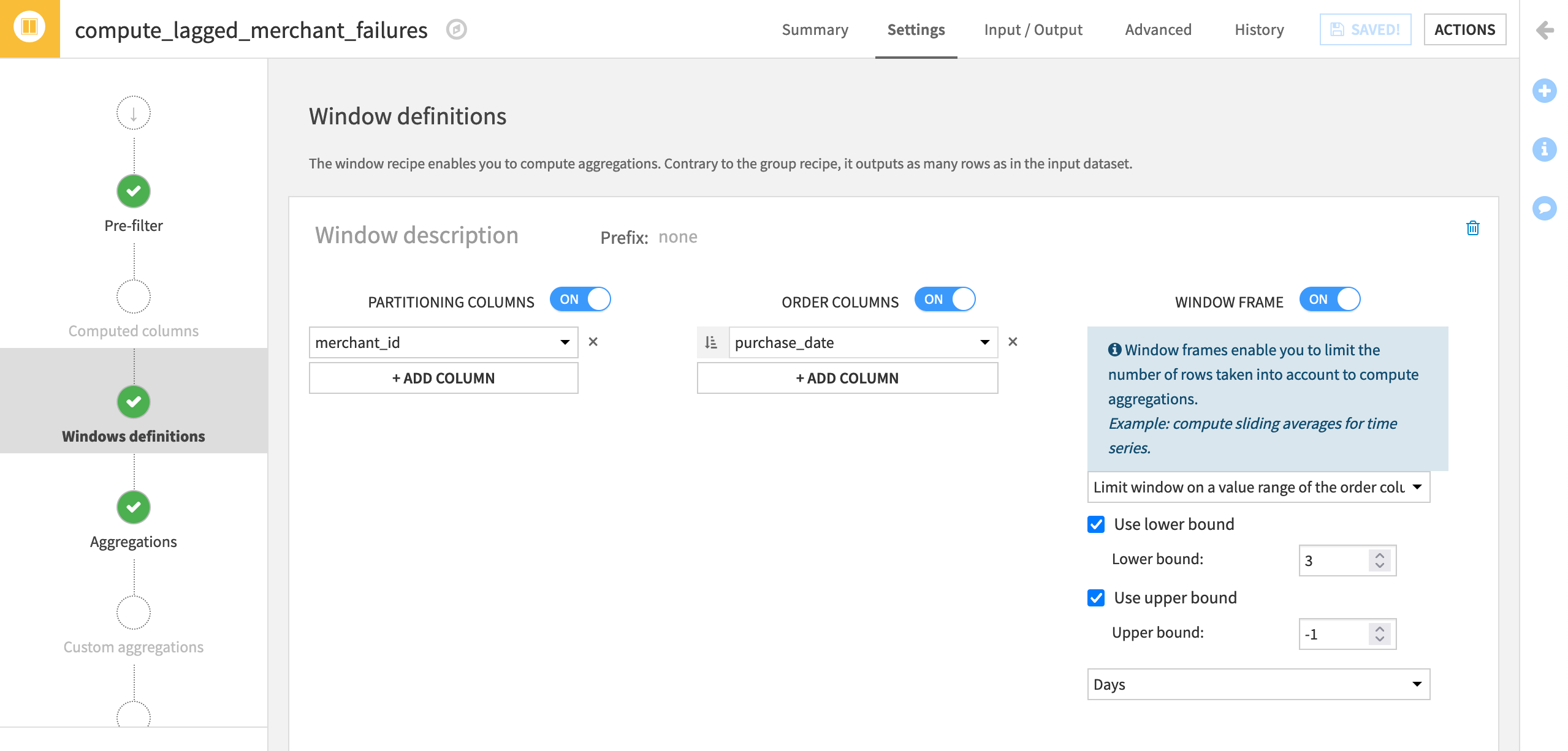
Our questions concern merchants and time so this determines our partitioning and order columns.

• On the Window definitions step, add merchant_id instead of card_id as the Partitioning Column.

• Add purchase_date in ascending order as the Order Column to put transactions in chronological order (per merchant_id).

• We’ll use the same Window Frame as the previous example. Limit the window on the order column with a lower bound of 3 days and an upper bound of -1 to exclude the present day.

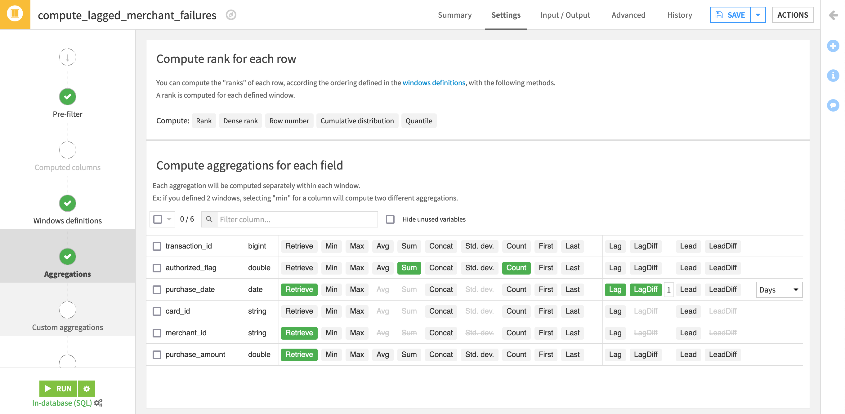
Now let’s move on to the aggregations.

• For simplicity, turn off Retrieve for unneeded columns: transaction_id, authorized_flag, and card_id.

• Include the following four aggregations:

  • the “Sum” of authorized_flag as a sanity check (it should always be 0 if our pre-filter is working);

  • the “Count” of authorized_flag to report the number of failed transactions for that merchant within the window frame;

  • the “Lag” of purchase_date to report the date of that merchant’s last failed transaction (the default offset of 1 is correct);

  • the “LagDiff” of purchase_date in days to report the number of days since that merchant’s last failed transaction.

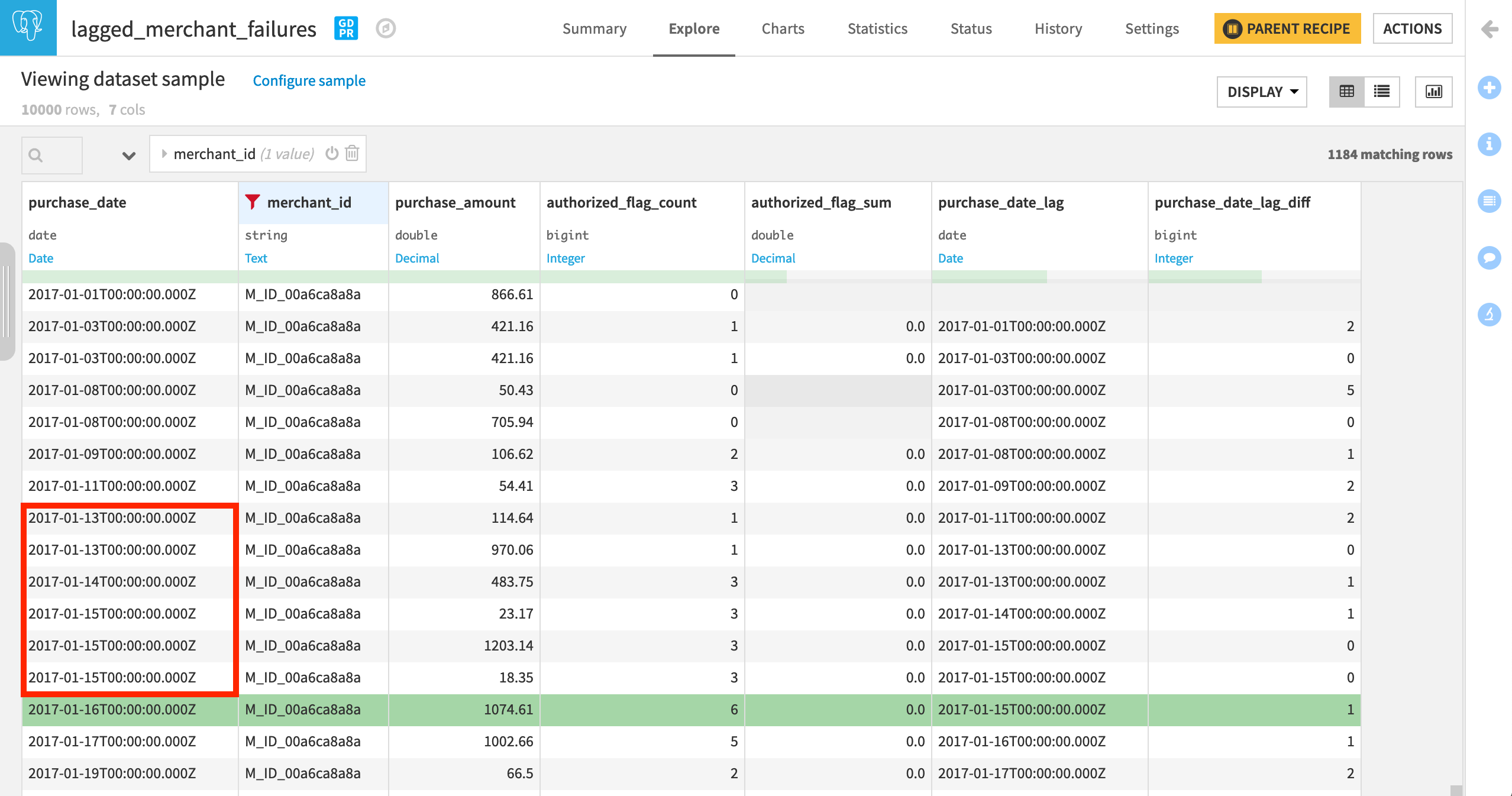
After running the recipe, explore the output dataset, and apply a filter for one merchant_id. Confirm the following for yourself:

• Rows are in increasing chronological order for every distinct merchant.

• After the pre-filter, the column authorized_flag should always be 0, and so its sum should also be 0.

• purchase_date_lag is the date of the previous row. Having access to a lagged value can be useful on its own or for further manipulation in a Formula step later.

• purchase_date_lag_diff is the difference between the date of the previous and present rows. We could have calculated this ourselves with purchase_date and purchase_date_lag in a Custom Aggregation or Formula, but the LagDiff function saves us the trouble.

To give one specific example, on Jan 16, the three prior days (13, 14, 15) had a combined six transactions that failed authorization!

What’s Next?

The Window recipe opens a world of possibilities. As shown here, it can be used to add grouped calculations as a column, compute cumulative sums or moving averages, as well as lagging differences.

You can get even more practice with another Window recipe tutorial in this article.