Hands-On Tutorial: Window Recipe

A window function is an analytic function, typically run in SQL and SQL-based engines (such as Hive, Impala, and Spark), which allows one to perform aggregate calculations across a set of table rows, while retaining the same row structure.

Some examples of computations that can be performed using a window function are moving averages, cumulative sums, and rankings.

The visual Window recipe in Dataiku allows you to take advantage of this powerful function without coding.

Windowing in Dataiku Concept Recap

The Window recipe is different from the Group recipe. The Window recipe groups your rows together, but instead of reducing the rows to just the aggregated rows, it keeps all of the rows and organizes them into a window frame based on how you configure it.

Conceptually, there are two steps when defining a window recipe:

• Defining the window(s): On what rows of the dataset will the computations apply?

• Defining the aggregation(s): What should be computed on this window?

The window can be partitioned, ordered, or bounded (framed):

• Partitioned: Define one or several columns, and one window is created for each combination of values of these columns.

• Ordered: Define one or several columns to order the windowed rows by (typically a date, a ranking, etc.).

• Bounded: For each row, restrict the window to only take into account the following:

  • a given number of rows before or after the current row

  • based on a given range of values that the window is ordered by (it’s therefore required to order the window in order to be able to bound it)

Note

Note that in Dataiku, the window bounding step is referred to as creating a “window frame”.

Let’s Get Started

The learning objectives for this hands-on tutorial are to:

• use the Window recipe to compute new potential features;

• apply a Post-filter step within a visual recipe;

• insert a recipe (and its output) into the middle of an existing Flow.

To achieve these objectives, we’ll work through a basic credit card fraud use case found in all tutorials in the Advanced Designer learning path. This binary classification problem uses a dataset of both labeled transactions known to have passed or failed authorization, as well as unknown transactions.

Advanced Designer Prerequisites

This lesson assumes that you have basic knowledge of working with Dataiku DSS datasets and recipes.

Note

If not already on the Advanced Designer learning path, completing the Core Designer Certificate is recommended.

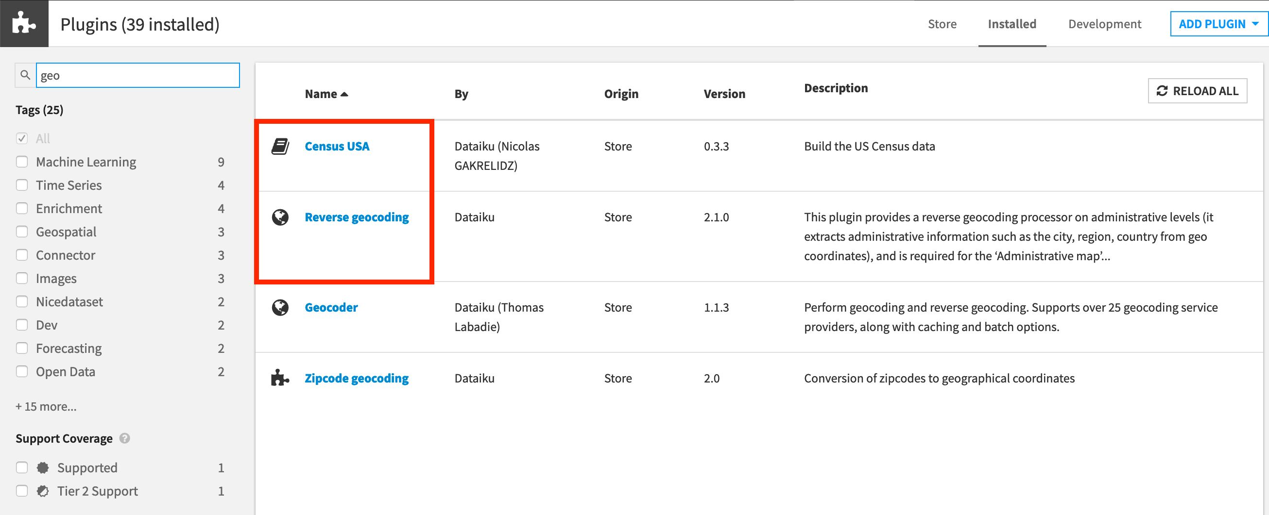
To complete the Advanced Designer learning path, you’ll need access to an instance of Dataiku DSS (version 8.0 or above) with the following plugins installed:

• Census USA (minimum version 0.3)

• Reverse geocoding

These plugins are available through the Dataiku Plugin store, and you can find the instructions for installing plugins in the reference documentation. To check whether the plugin is already installed on your instance, go to the Installed tab in the Plugin Store to see a list of all installed plugins.

Note

If your goal is to complete only the tutorials in Visual Recipes 102, the Census USA plugin is not required.

Plugin Installation for Dataiku Online Users

Tip

Users of Dataiku Online should note that while plugin installation is not directly available, you can still explore available plugins from your launchpad:

• From your instance launchpad, open the Features panel on the left hand side.

• Click Add a Feature and choose “US Census” from the Extensions menu. (“Reverse geocoding” is already available by default).

• You can see what plugins are already installed by searching for “installed plugins” in the DSS search bar.

In order to get the most out of this lesson, we recommend completing the following lessons beforehand:

• Concept: Window Recipe

• Concept: Common Steps in Recipes

Workflow Overview

In this tutorial, we’ll be creating new features in a Window recipe, and then inserting the recipe’s output into an existing Flow so these features are available for the machine learning task downstream (predicting which credit card transactions are potentially fraudulent).

Create Your Project

• From the Dataiku homepage, click +New Project > DSS Tutorials > Advanced Designer > Window Recipe (Tutorial).

Note

You can also download the starter project from this website and import it as a zip file.

Change Dataset Connections (Optional)

Aside from the input datasets, all of the others are empty managed filesystem datasets.

You are welcome to leave the storage connection of these datasets in place, but you can also use another storage system depending on the infrastructure available to you.

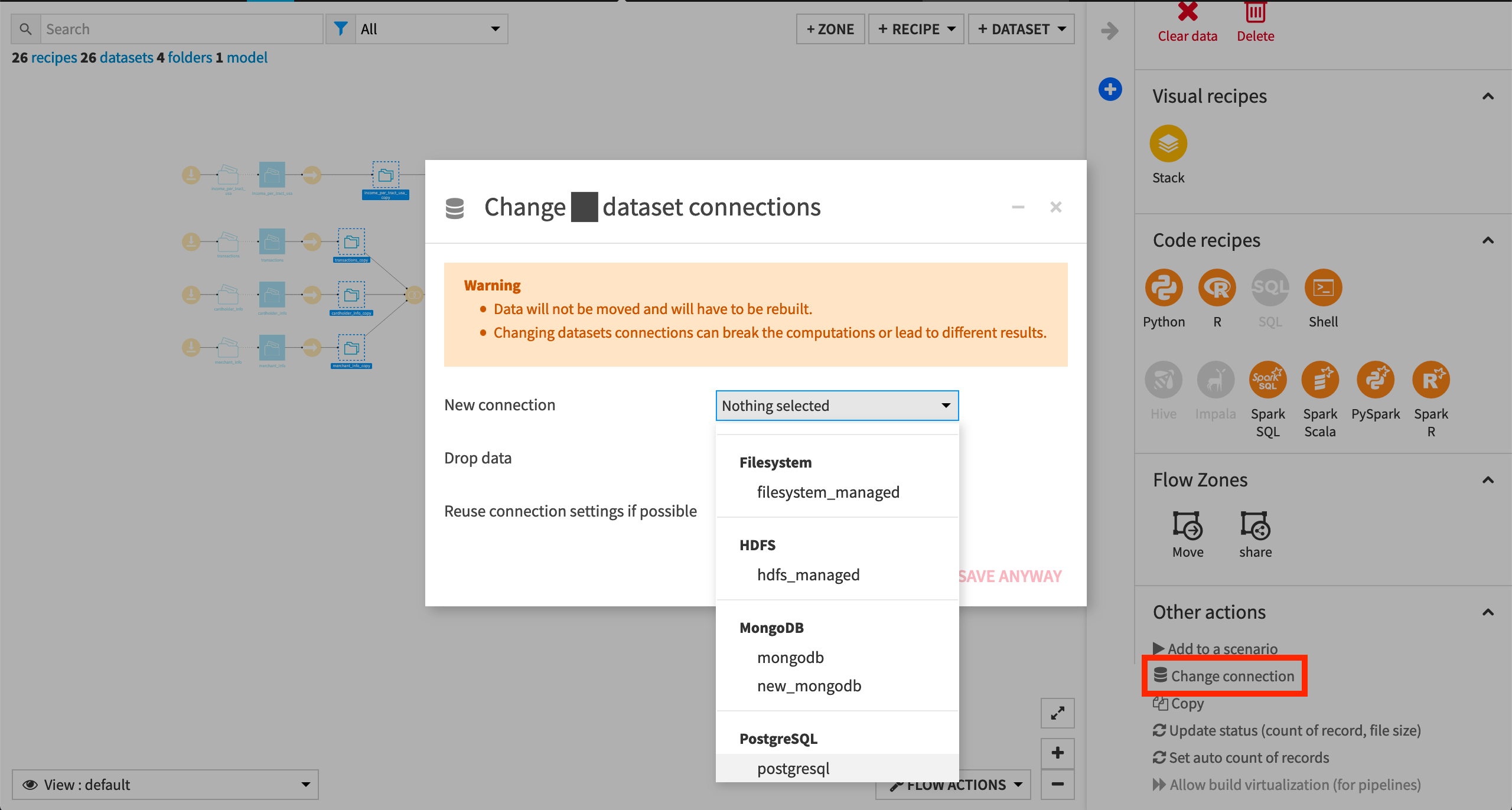
To use another connection, such as a SQL database, follow these steps:

• Select the empty datasets from the Flow. (On a Mac, hold Shift to select multiple datasets).

• Click Change connection in the “Other actions” section of the Actions sidebar.

• Use the dropdown menu to select the new connection.

• Click Save.

Note

For a dataset that is already built, changing to a new connection clears the dataset so that it would need to be rebuilt.

Note

Another way to select datasets is from the Datasets page (G+D). There are also programmatic ways of doing operations like this that you’ll learn about in the Developer learning path.

The screenshots below demonstrate using a PostgreSQL database.

• Build the branch of the Flow ending in the dataset transactions_unknown_scored.

See Build Details Here if Necessary

• From the Flow, select the end dataset required for this tutorial: transactions_unknown_scored

• Choose Build from the Actions sidebar.

• Choose Recursive > Smart reconstruction.

• Click Build to start the job, or click Preview to view the suggested job.

• If previewing, in the Jobs tab, you can see all the activities that Dataiku will perform.

• Click Run, and observe how Dataiku progresses through the list of activities.

Inspect the Advanced Designer Data

• Once your Flow is built, open the transactions_joined_prepared dataset.

The transactions_joined_prepared dataset contains information about credit card transactions. Each row represents one transaction, consisting of the following notable columns:

• transaction_id, the transaction’s ID

• purchase_date, the date of the transaction

• card_id, the credit card it was made with

• merchant_id, the merchant with whom the transaction was made

• purchase_amount, the amount of the transaction, and

• authorized_flag, the target variable of the ML task, which is a 1 if the transaction was authorized or a 0 if it failed authorization.

In this exercise, we will focus on creating aggregated statistics based on the purchase_amount column. These new columns could potentially be valuable features helping to predict which transactions will fail authorization.

• Analyze the purchase_amount column.

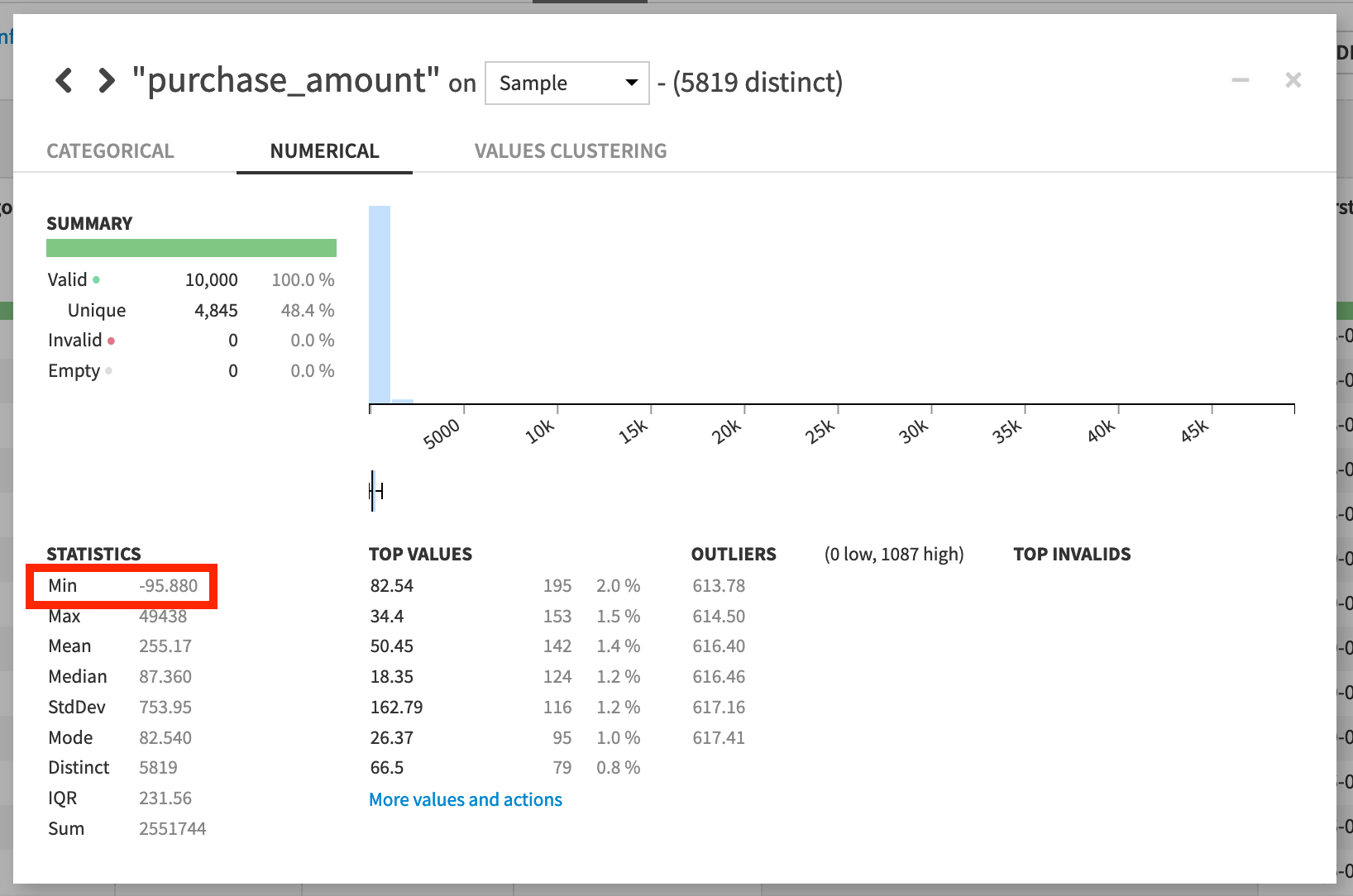
Whether analyzing the purchase_amount column over the entire dataset or just a sample, notice that there are negative values. This is because some rows represent refunds made by the merchant to the cardholder.

• Return to the Flow.

The transactions_joined_prepared dataset is split into two new datasets: transactions_known and transactions_unknown.

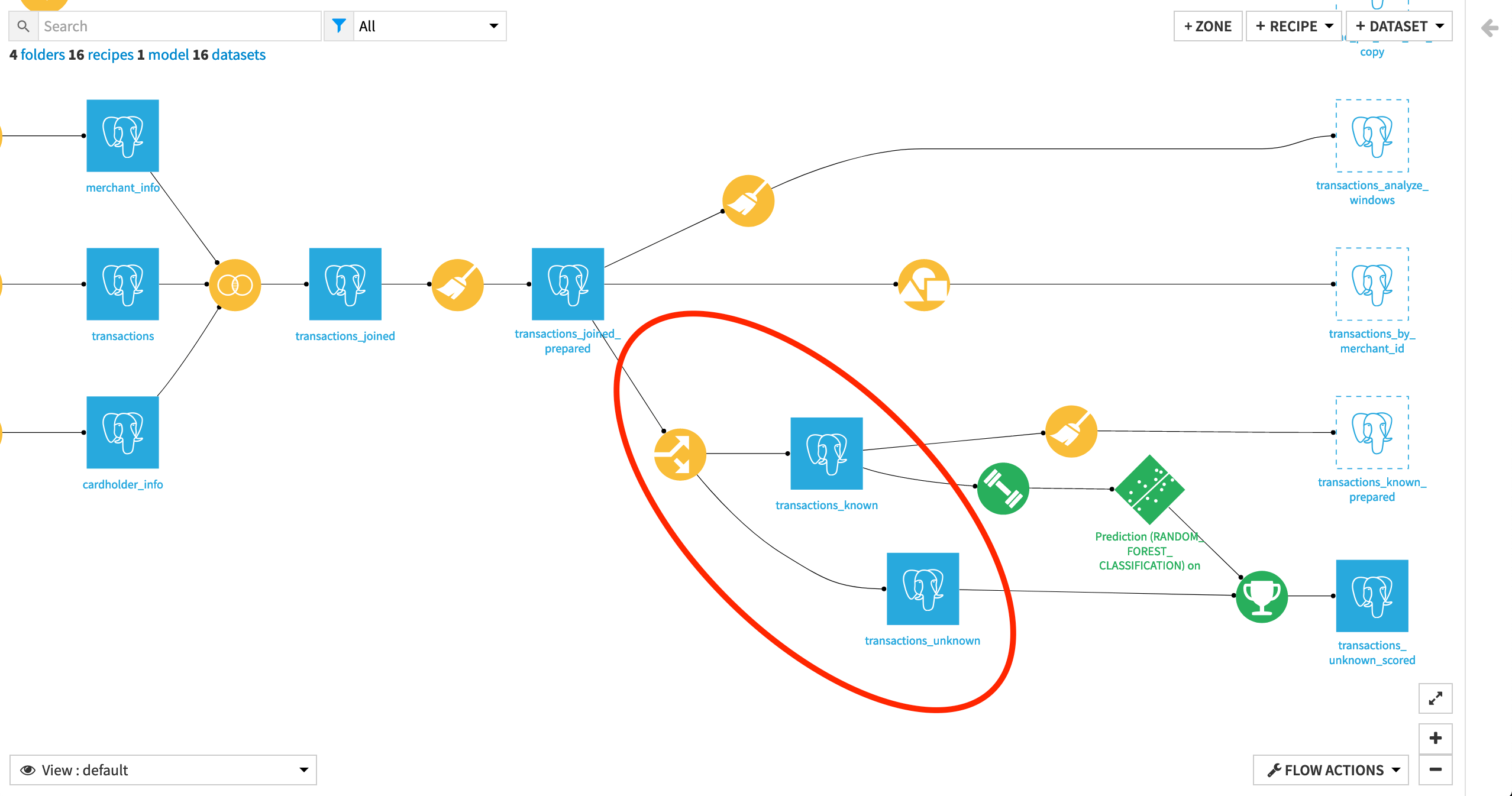
• Let’s explore the Split recipe.

Notice the dataset was split on the condition “authorized_flag is defined”. Thus, the transactions_known dataset contains all the transactions for which we know whether they were authorized or not, and transactions_unknown contains the ones for which the authorized_flag value is empty.

• Return to the Flow.

The transactions_known dataset is used to train a machine learning algorithm, which is then applied to the unknown transactions data in order to predict the value of the authorized_flag column. In other words, the known outcome in the training data is used to predict whether each unknown transaction was authorized or not.

To generate additional features for our machine learning model, we want to compute some row aggregations on the transactions_joined_prepared dataset, while keeping the structure of the dataset intact.

Formulate the Question

What kind of aggregations should we compute? On which groups? And over what kind of window?

We might want to know the minimum, maximum, and average purchase amount for every cardholder. We might want to know the same for every merchant. These kinds of questions we can answer with just a Group recipe.

However, we don’t have to settle for one single average (or max, min, sum, etc) for every cardholder (or merchant). The Window recipe allows us to calculate these kinds of aggregations for some group, for some particular window of rows.

For example, the Window recipe can tell us the average purchase amount for every cardholder during some time period with respect to the present transaction.

Note

In this case, let’s find the minimum, maximum, and average purchase amount for every cardholder (and for every merchant) at any point in time. That is, on any particular date, the aggregations will include all past transactions, but no future transactions from after that date.

Create the Window Recipe

With that question in mind, let’s get to work.

• From the transactions_joined_prepared dataset, select Actions > Window to create a new Window recipe.

• Name the output dataset transactions_windows.

For our first window, we are interested in computing aggregations by cardholder (i.e., to look at the total number of rows or the average of a given column value for each card ID). To do this:

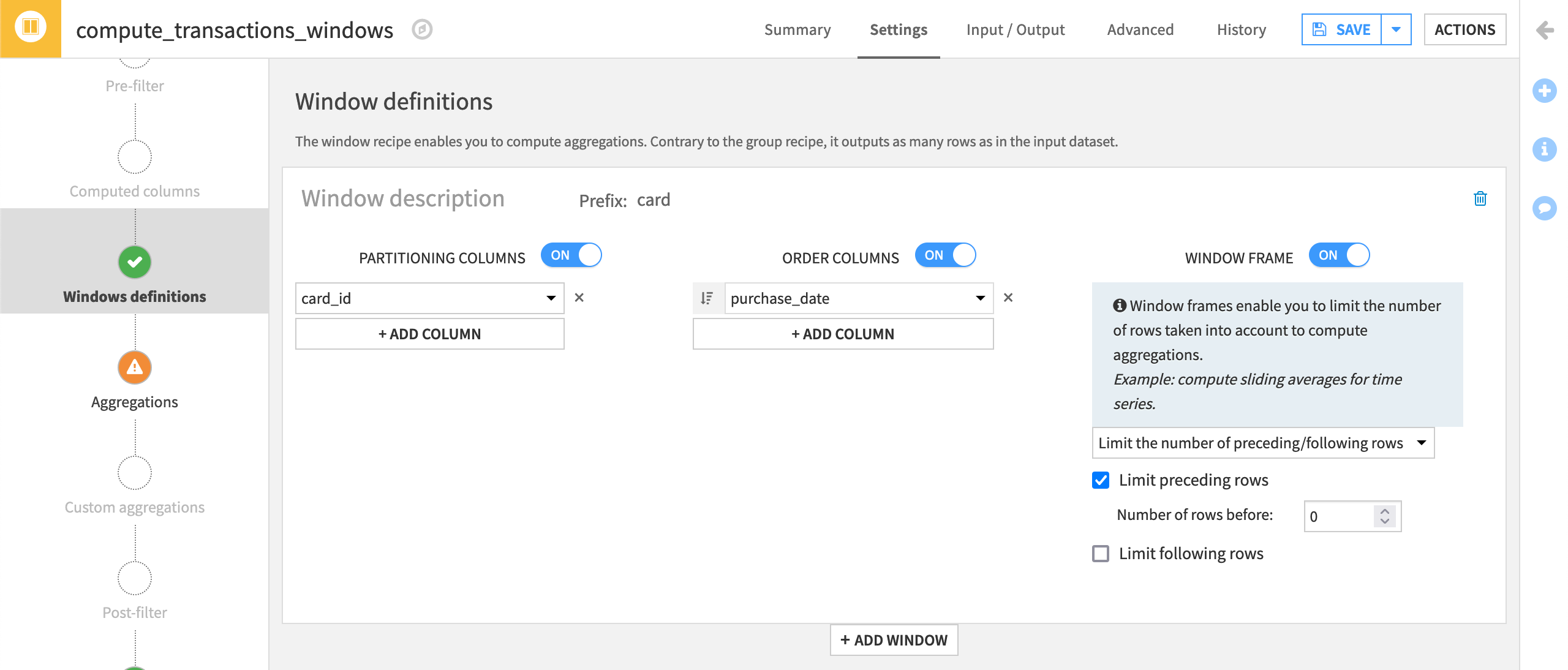
• On the Window definitions step, activate Partitioning Columns, and select card_id from the dropdown menu.

• Next, activate Order Columns.

This will allow you to order each grouping of aggregated rows by a certain criteria.

• Select purchase_date from the dropdown menu, and click on the sort icon to select descending order .

This way, when you look at all of the transactions for a given card in your output dataset, the most recent ones will display at the top.

• Finally, activate Window Frame.

Using a Window frame allows you to limit the number of rows taken into account to compute aggregations. Once activated, Dataiku DSS displays two options: “Limit the number of preceding/following rows” and “Limit window on a value range from the order column”.

• Leave the default selection “Limit the number of preceding/following rows”, and select Limit preceding rows.

We want the computed aggregations to take into account the prior transactions, but because we have ordered the transactions by purchase dates in descending order, “the preceding rows” correspond to the more recent transactions than the current one, so we need to exclude those.

For example, if we were to compute the sum of all purchase amounts by card_id, and look at a transaction made on “2017-02-06”, the sum would only reflect purchases made up to that point.

Note

If we were to select Limit window on a value range from the order column, we would be limiting the number of rows to compute aggregations based on the order column. For example, if we selected to order by date, we could choose to only compute aggregations on the transactions from the past six months.

• Finally, since we are going to define two windows in this recipe, add the prefix card to make the aggregated columns easier to recognize.

Compute Aggregated Statistics

With this window in place, let’s define our aggregations to compute.

• On the left hand panel, click on Aggregations.

Here you can select the columns you want to retrieve and compute aggregations on. At the moment, all of the columns from the input dataset are selected by default to be retrieved in the output dataset. Let’s retrieve these, and compute some additional columns.

• Find the purchase_amount column, and select to compute the Min, Max, and Avg.

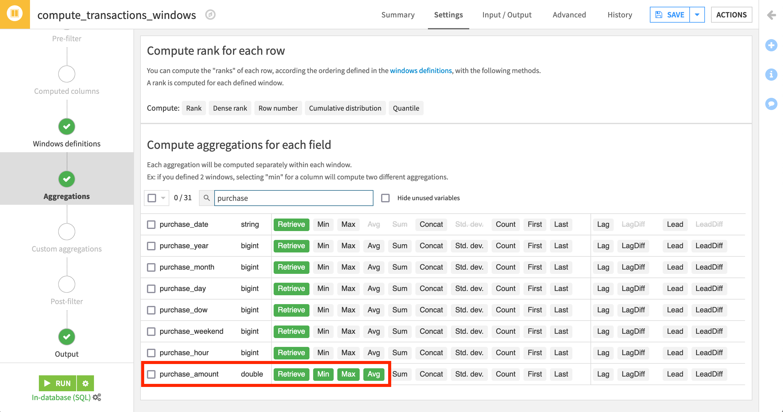
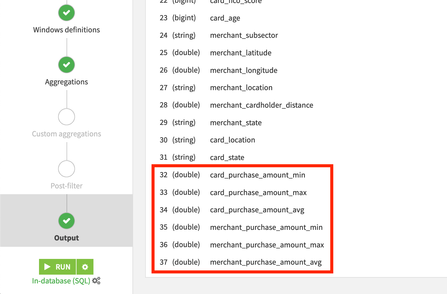
This will create three new columns in the output dataset. You can verify this by going to the Output step from the left menu:

• card_purchase_amount_min,

• card_purchase_amount_max,

• and card_purchase_amount_avg

representing the minimum, maximum, and average purchase amount for all transactions belonging to a card ID up to and including the present date.

• Before running it, Save and update the schema of the output dataset.

Create Multiple Windows in One Recipe

Let’s say we want to look at the same statistics–minimum, maximum, and average of the purchase amount–but this time we want them grouped by merchant instead of by card ID. It would be useful to have both the aggregations by card and by merchant appear in the same output dataset, so that we can compare them and potentially use them as features in our machine learning model.

You could create a new Window recipe from the output dataset of this one, but it would be easier and faster to do it as part of the same recipe–Dataiku DSS allows us to do that.

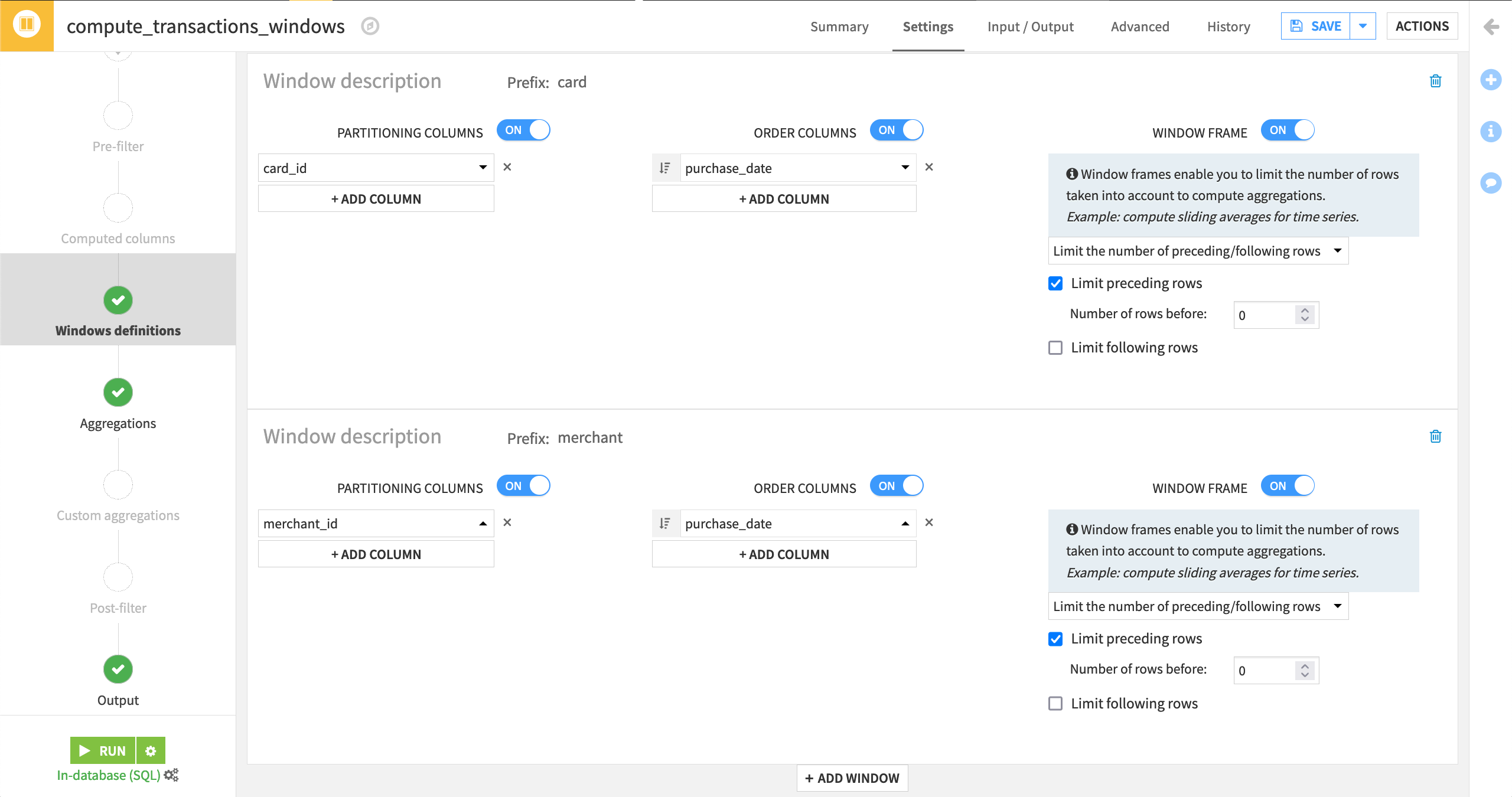
• Go back to Windows definitions step, and click on + Add Window.

• Activate Partitioning Columns, and this time select merchant_id.

• Activate Order Columns, ordering by purchase_date in descending order.

• Activate Window Frame, limiting the preceding rows to be taken into account to 0.

• Give this window the prefix merchant.

You can verify that the output columns all contain the correct prefix and are understandable to you (or, if not, change their names) in the Output step:

• Save and update the output schema once more.

Apply a Post-Filter in a Visual Recipe

Finally, instead of applying a separate Filter recipe after the Window, let’s filter our results within the Window recipe itself. Here, let’s only keep rows in which the average purchase amount by card ID is positive.

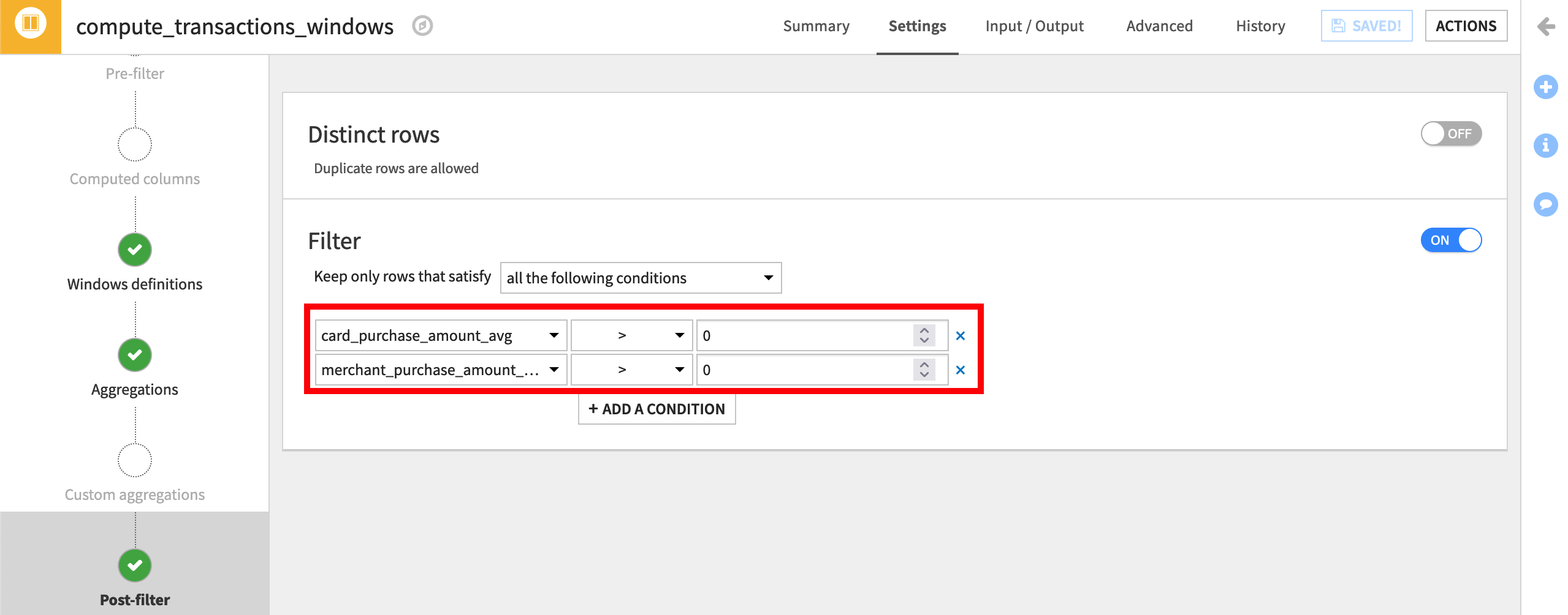
• Click on Post-filter on the left menu, and then activate the filter.

• Select Keep only rows that satisfy “all the following conditions” where the card_purchase_amount_avg column is “>” 0.

Note

Many visual recipes offer the option of pre- and post-filter steps in addition to windowing, grouping, joining, splitting, etc. Whether a pre- or post-filter step is the right choice depends on a variety of factors, such as transparency, efficiency, and Flow management.

You can add a similar condition for the purchase amount average by merchant.

• Click on + Add Condition, and select merchant_purchase_amount_avg “>” 0.

• Then Run the recipe.

Explore the Output Dataset

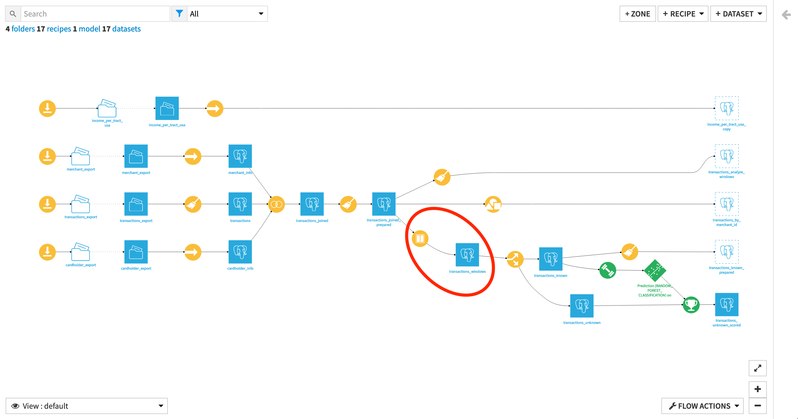
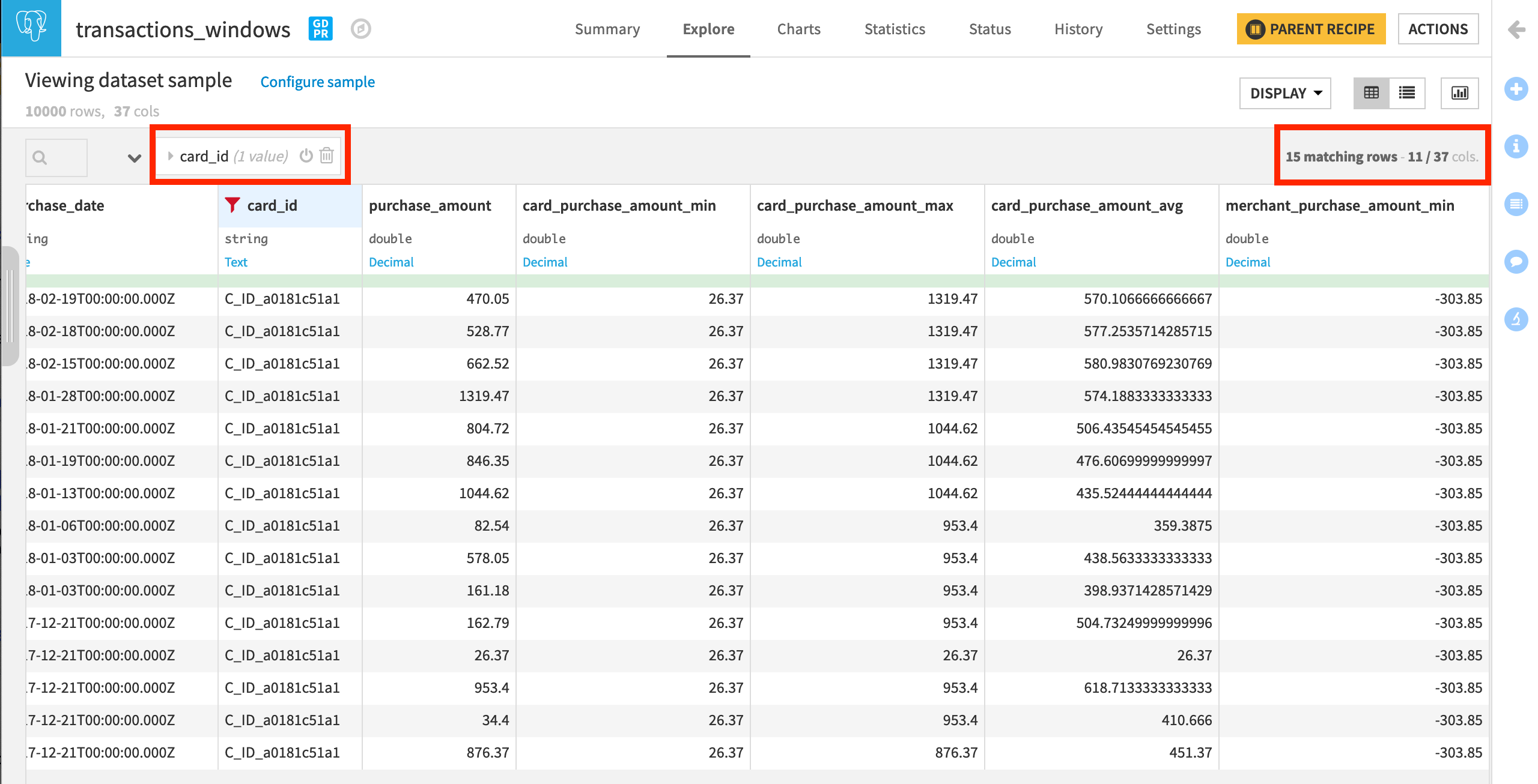
• Click on Explore transactions_windows to open the output dataset.

Notice there are six new columns, each containing aggregated statistics about the minimum, maximum, and average purchase amount by card and by merchant respectively, and ordered by date in descending order.

• To verify this, click on the card_id column, and select Filter from the dropdown menu.

• Check one of the card ID boxes to display all the transactions made with one particular credit card.

Tip

Compare the max or min columns to the purchase_amount column to verify for yourself which rows have been included in the window frame.

Change the Input Dataset of a Recipe

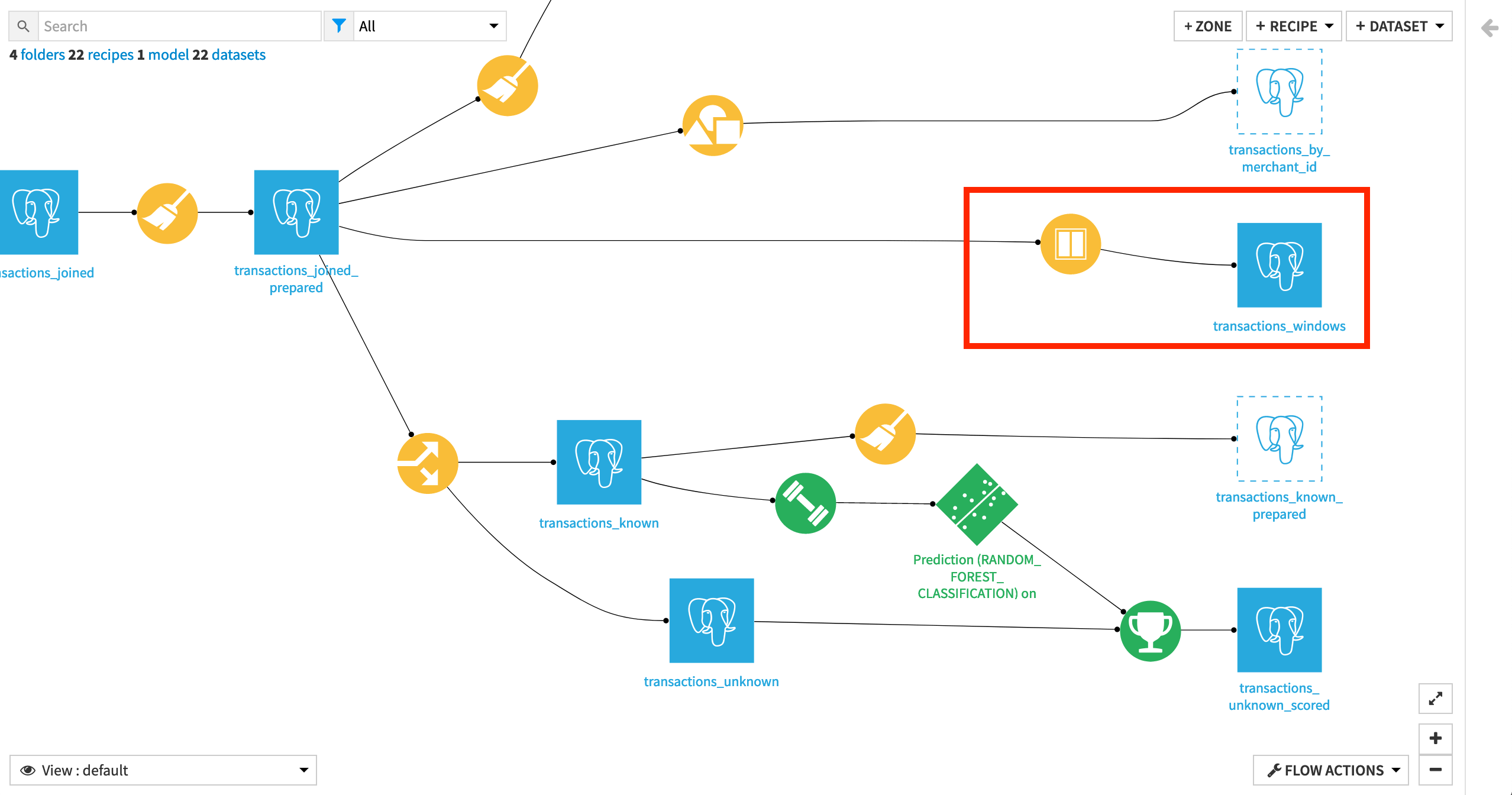
The last objective of this tutorial is to compute aggregated statistics using the Window recipe to generate additional potential features for the machine learning model. However, the output dataset transactions_windows is currently part of a separate branch, or subflow, that is not upstream of the machine learning branch of the Flow.

We can fix this by changing the input dataset of the Split recipe (which marks the beginning of the machine learning subflow) to be the transactions_windows dataset. To do this:

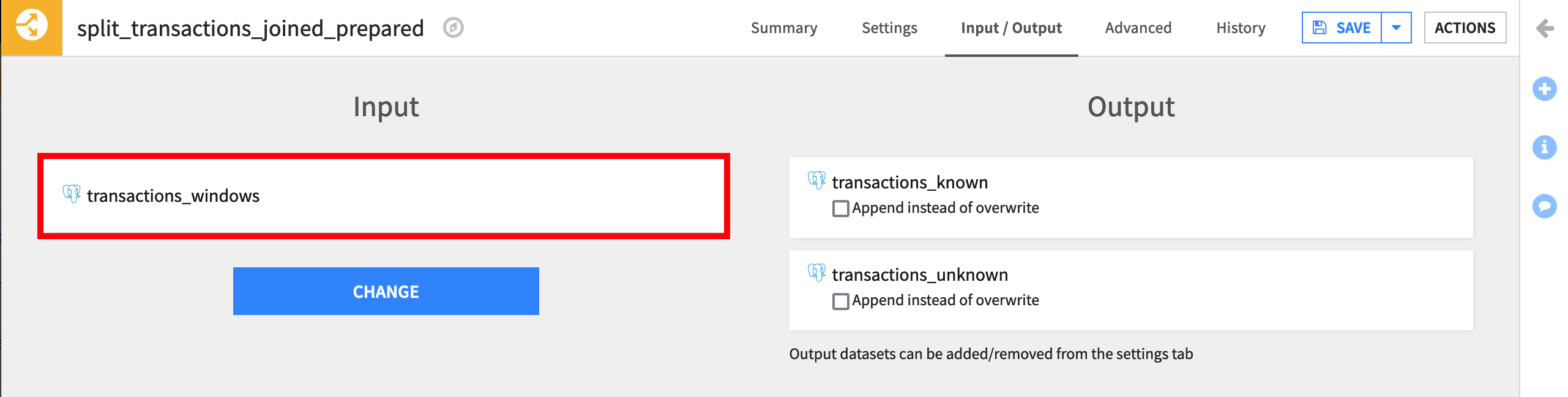
• Open the Split recipe, and navigate to the Input / Output tab.

• Under Input, click on Change, and then select transactions_windows.

Handling Downstream Schema Changes

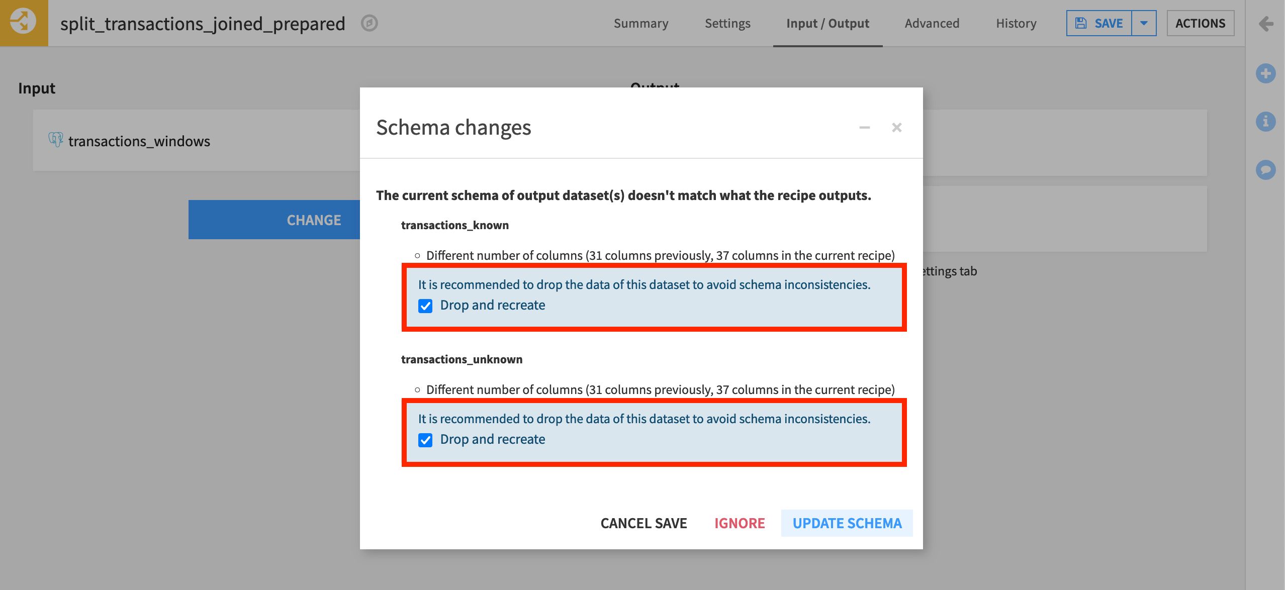
When you click Save after changing the input dataset to the Split recipe, pay close attention to the schema change notification.

Dataiku has detected a change in the number of columns, and so recommends to drop and recreate the two output datasets.

• Leave the box for “Drop and recreate” checked, and click Update Schema.

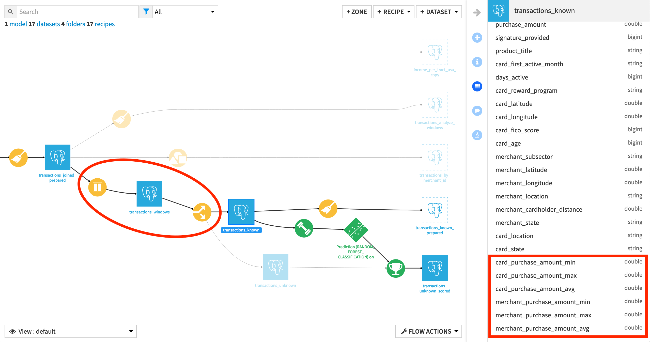
Returning to the Flow, notice three things:

• The output dataset from the Window recipe is now the input dataset for the Split recipe.

• The Split recipe output datasets transactions_known and transactions_unknown have the six new columns included in their schema.

• Further downstream datasets transactions_known_prepared and transactions_unknown_scored do not.

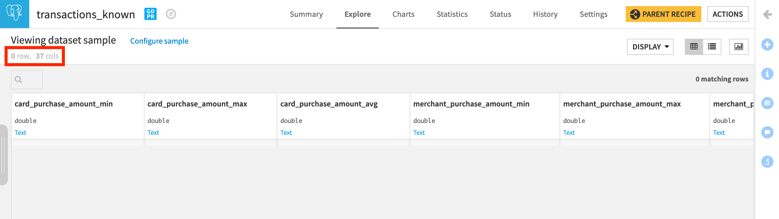
Also, if you open transactions_known or transactions_unknown, you’ll find that they now have 37 columns (instead of the original 31), but they have 0 rows. This is because we accepted the drop and recreate option in the schema update.

These datasets will need to be rebuilt if we actually want to use these features in model training!

Note

You’ll learn more about schema propagation in the Flow Views & Actions course.

Summary & Next Steps

In this lesson, you learned how to:

• create a Window recipe to compute aggregated statistics on a subset (or partition) of your data while keeping the same number of rows;

• add multiple windows as part of the same Window recipe;

• apply a post-filter step to a visual recipe;

• change the input dataset of a recipe.

In the optional Window Recipe: Deep Dive hands-on, you can apply your knowledge to even more advanced usages of the Window recipe.