Hands-On Tutorial: Dataiku DSS for R Users (Advanced)
Dataiku DSS is a collaborative data science and machine learning platform. Its visual tools enable collaboration with a wider pool of colleagues who may not be coders (or R coders for that matter). At the same time, code integrations for languages like Python and R retain the flexibility needed when greater customization or freedom is desired.
Over the course of this hands-on tutorial, you’ll recreate a simple Flow built with visual tools using the integrations designed for R users.
Tip
You can also find this tutorial as part of the Academy course on Dataiku DSS for R Users, which is part of the Developer learning path.
Let’s Get Started
In this hands-on tutorial, you’ll learn how to:
build an ML pipeline from R notebooks, recipes, and project variables;
apply a custom R code environment to use CRAN packages not found in the base environment;
use the DSS R API to edit DSS recipes and create ggplot insights from within RStudio;
import R code from a git repository into a DSS project library; and
work with managed folders to handle file types such as “*.RData”.
Prerequisites
To complete this tutorial, you’ll need:
basic Dataiku DSS knowledge;
access to a Dataiku DSS instance (version 8.0 or above) with the R integration installed;
an R code environment with the packages tidyr, ggplot2, gbm, and caret (or the permission to create a new code environment);
RStudio Desktop integration (optional).
Workflow Overview
When you have completed the tutorial, you will have built the bottom half of the Flow pictured below:
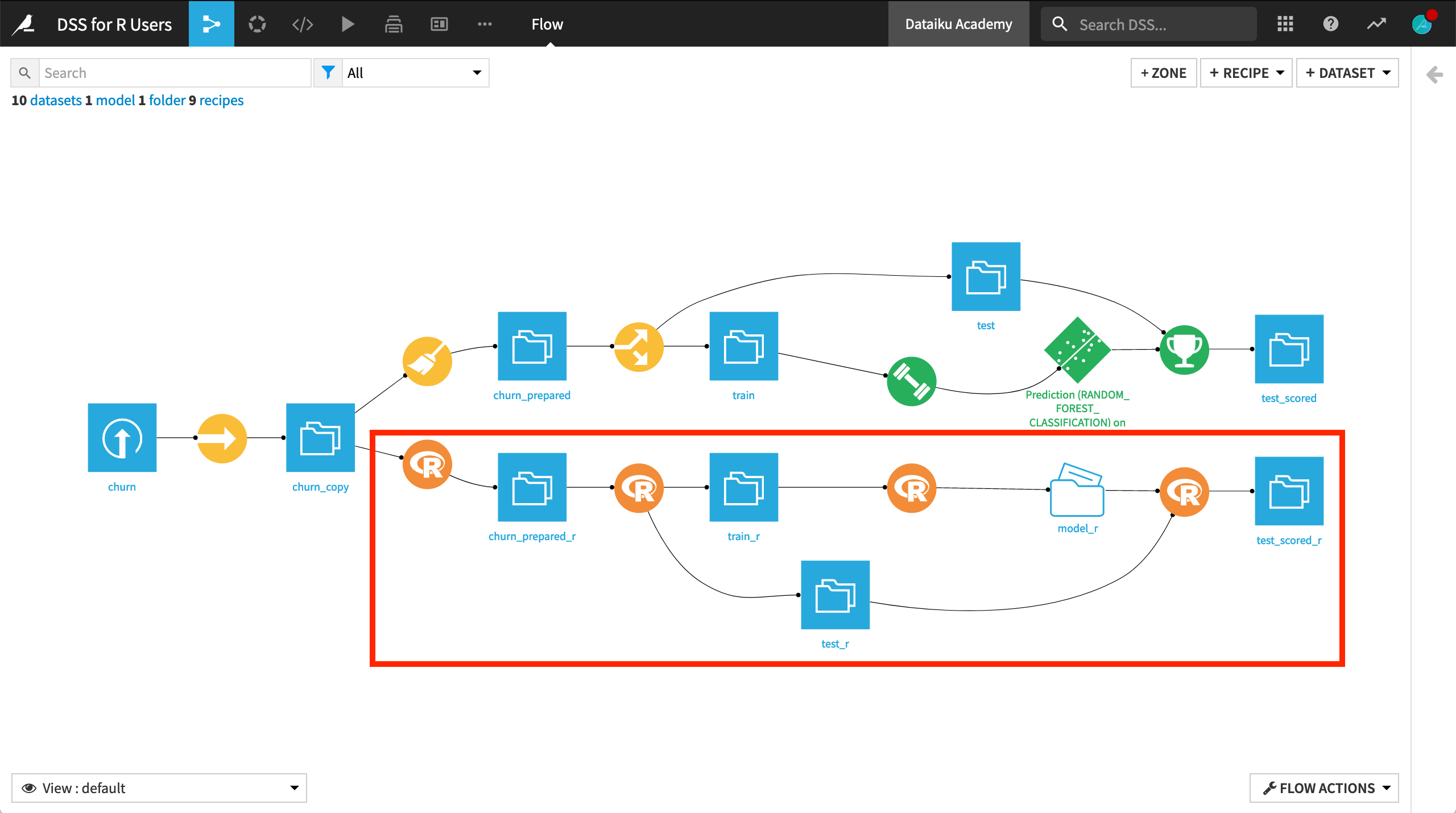
Create the Project
We’ll start with a project built entirely with visual tools:
The data pipeline consists of visual recipes.
The native Chart builder has been used for exploratory visualizations.
The machine learning model (shown in green) has been built with the visual ML interface.
Although using visual tools can amplify collaboration and understanding with non R-coding colleagues, re-creating this Flow in R opens windows for greater flexibility and customization at every stage.
From the Dataiku DSS homepage, click on +New Project > DSS Tutorials > Developer > Dataiku DSS for R Users.
Note
You can also download the starter project from this website and import it as a zip file.
After creating the project, go to the Flow, and click Build all > Build from the Flow Actions menu in the bottom right corner.
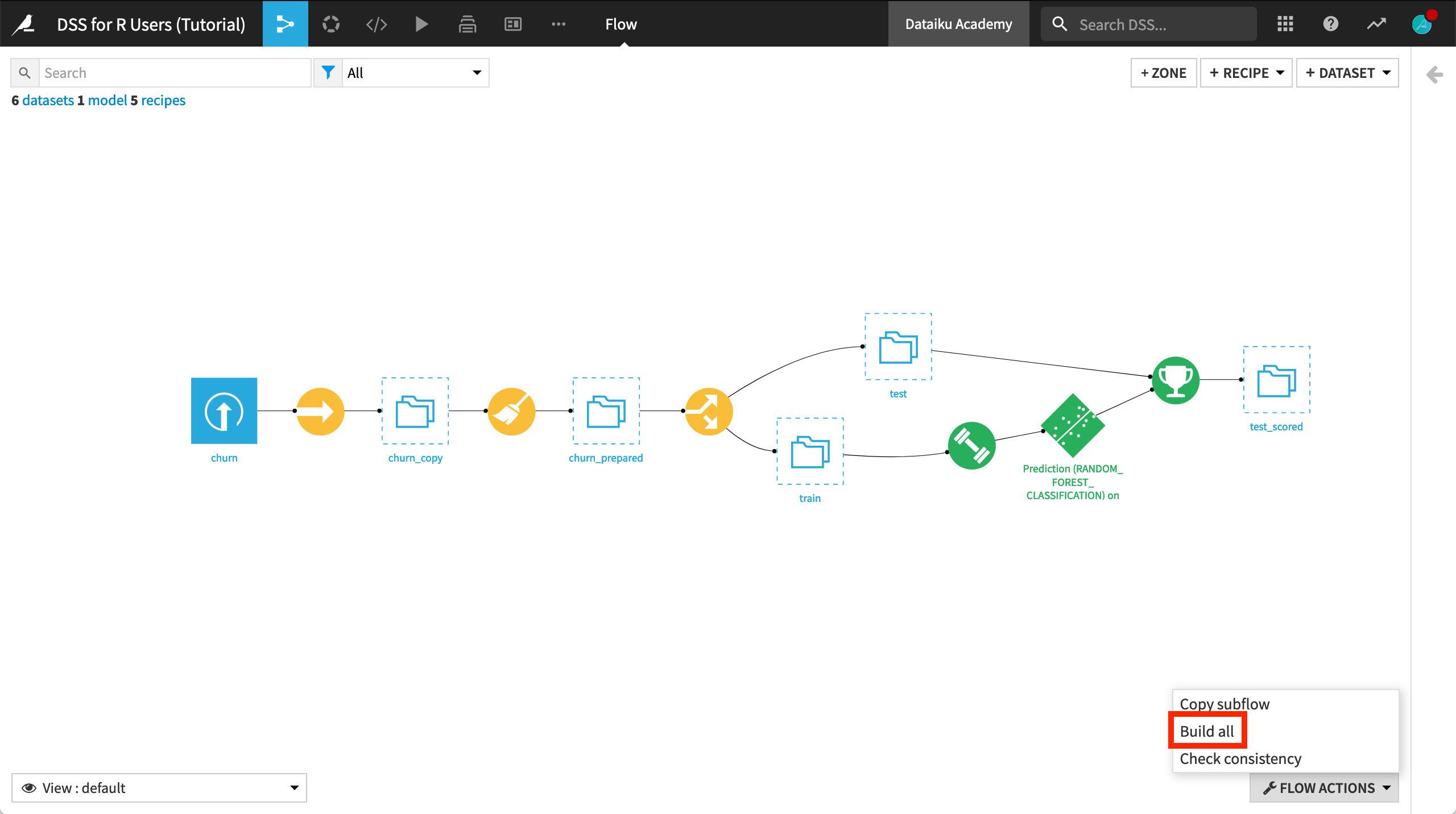
Observe the Visual Flow
Even if primarily an R user, it will be helpful for you to familiarize yourself with the available set of visual recipes and what they can achieve.
Although the table below is far from 1-1 matching, it suggests a Dataiku DSS recipe that performs a similar operation for some of the most common data preparation functions in base R or the tidyverse.
R package |
R function |
Similar Dataiku DSS recipe |
|---|---|---|
dplyr |
mutate() |
Formulas in Prepare recipe |
dplyr |
select() |
Delete/Keep processor in Prepare recipe |
dplyr |
filter() |
|
dplyr |
arrange() |
Sort recipe |
dplyr |
group_by() %>% summarize() |
Group recipe |
dplyr |
group_by() %>% mutate() |
Window recipe |
dplyr |
*_join() |
Join recipe |
dplyr |
distinct() |
Distinct recipe |
tidyr |
gather() / pivot_longer() |
Fold multiple columns processor in Prepare recipe |
tidyr |
spread() / pivot_wider() |
Pivot recipe Pivot processor in Prepare recipe |
base, dplyr |
rbind(), bind_rows() |
Stack recipe |
base, dplyr |
subset(), group_split() |
Split recipe |
base, dplyr |
head/tail(), slice_min/max() |
Top N recipe |
stringr |
NA |
String processors in Prepare recipe |
lubridate |
NA |
Date processors in Prepare recipe |
fuzzyjoin |
NA |
Fuzzy Join recipe |
Note
As shown in the table, processors found in the Prepare recipe handle many data preparation functions. Moreover, many recipes and processors–although having a visual interface on top–are SQL-compatible.
Create an R Recipe
If you look at the Prepare recipe that creates the churn_prepared dataset, you’ll see it contains only a few simple steps. For routine data preparation, a visual recipe is an excellent choice since a wider pool of colleagues can more easily understand the actions in the Flow.
That being said, an R recipe grants you the freedom to code as you wish.
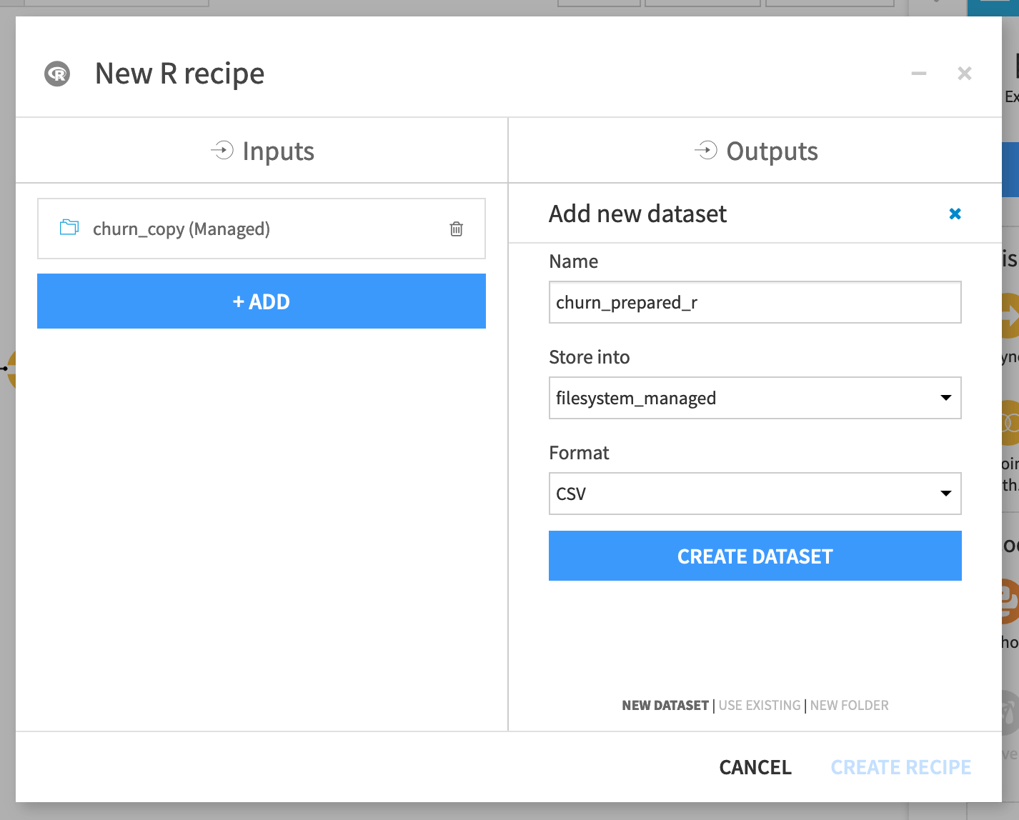
From the churn_copy dataset, add an R recipe from the Actions sidebar on the right.
Name the output dataset
churn_prepared_r.Click Create Dataset and Create Recipe.
Let’s break down the default R code recipe.
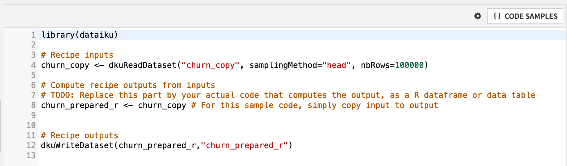
The first line loads the dataiku R package, which includes functions for interacting with DSS objects, such as datasets and folders.
Two functions from this package are included in the default recipe: dkuReadDataset() and dkuWriteDataset(). These functions simplify the process for reading and writing datasets.
The churn_copy dataset, in this case, is a managed filesystem dataset, resulting from the original uploaded CSV file. However, if the Sync recipe were instead moving the CSV file to an SQL database or an HDFS cluster, the syntax in the R recipe would be exactly the same.
The line churn_prepared_r <- churn_copy assigns the input dataset as the output dataset. You’ll want to replace this with your own logic to define a new output dataset based on the input.
Note
dkuReadDataset() is not the only way to read a dataset with R. dkuSQLQueryToData() makes it possible to execute SQL queries from R. This can be helpful when you want to pull in a specific query of records into Dataiku DSS, rather than any of the standard sampling options.
Code in an R Notebook
The recipe editor does not allow you to interactively test your code. Native Jupyter notebooks serve that purpose.
From the compute_churn_prepared_r recipe editor, click Edit in Notebook.
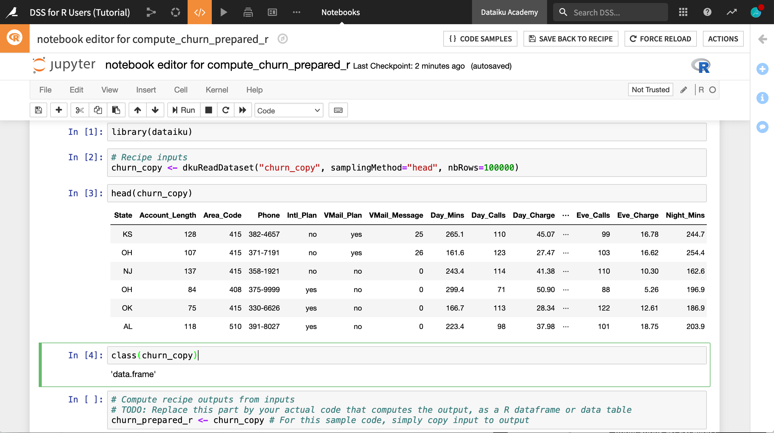
The recipe exists now in one cell of a Jupyter notebook with an R kernel.
For convenience, click Edit > Split Cell, or use the keyboard shortcut
Ctrl+Shift+-, to divide the recipe into four cells as shown below.Run the first two cells so that churn_copy is an in-memory dataframe.
Add a new cell underneath churn_copy’s local creation, and run commands like
head(churn_copy)andclass(churn_copy)to test this out.
Tip
To learn more about code notebooks, you may wish to register for the Academy course, Code in Dataiku DSS.
The R Code Environment
Notice that the kernel of this notebook in the upper right corner says “R”. This means that the notebook is using the default R code environment for this instance.
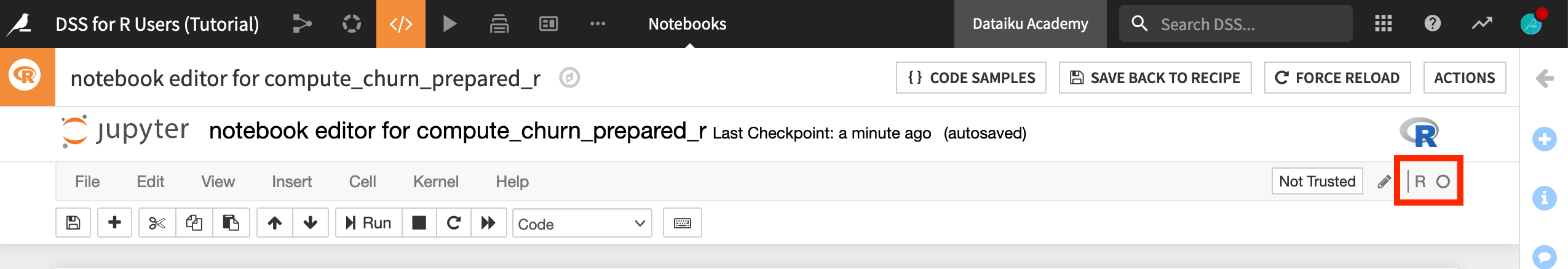
Accordingly, in addition to base R commands like head() and class(), you can also load and use functions from packages included in this environment.
Add a new cell, and run the command
library()$results[,1]to see a list of installed packages in the current environment.
You’ll find that dplyr is one base package. Let’s use it in this recipe.
Delete the existing recipe and any exploratory code.
Copy and paste the code below to mimic some of the steps of the visual Prepare recipe.
library(dataiku)
library(dplyr)

# Recipe inputs
churn_copy <- dkuReadDataset("churn_copy", samplingMethod="head", nbRows=100000)

# Data preparation
churn_copy %>%
    rename(Churn = Churn.) %>%
    mutate(Churn = if_else(Churn == "True.", "True", "False"),
        Area_Code = as.character(Area_Code)) %>%
    select(-Phone) ->
    churn_prepared_r

# Recipe outputs
dkuWriteDataset(churn_prepared_r,"churn_prepared_r")
Click Save Back to Recipe.
Once in the recipe editor, click Run.
Tip
You’ll find a more conceptual look at what code environments achieve in the Code in Dataiku DSS Academy course.
Change the R Code Environment
In many cases, you’ll want to use R packages not found in the base environment of the instance. In these cases, you’ll need to use a code environment that includes these packages.
For this project, we’ll need the following R packages:
tidyr (for data preparation),
ggplot2 (for visualization), and
gbm and caret (for machine learning).
Note
The product documentation includes instructions for creating a new R code environment. Follow these instructions, and add “tidyr”, “ggplot2”, “gbm” and “caret” as the requested packages. If you don’t have the requisite permissions, you’ll need to contact your DSS administrator.
When you have a code environment on your instance with at least these four additional R packages, you can activate it in the current project.
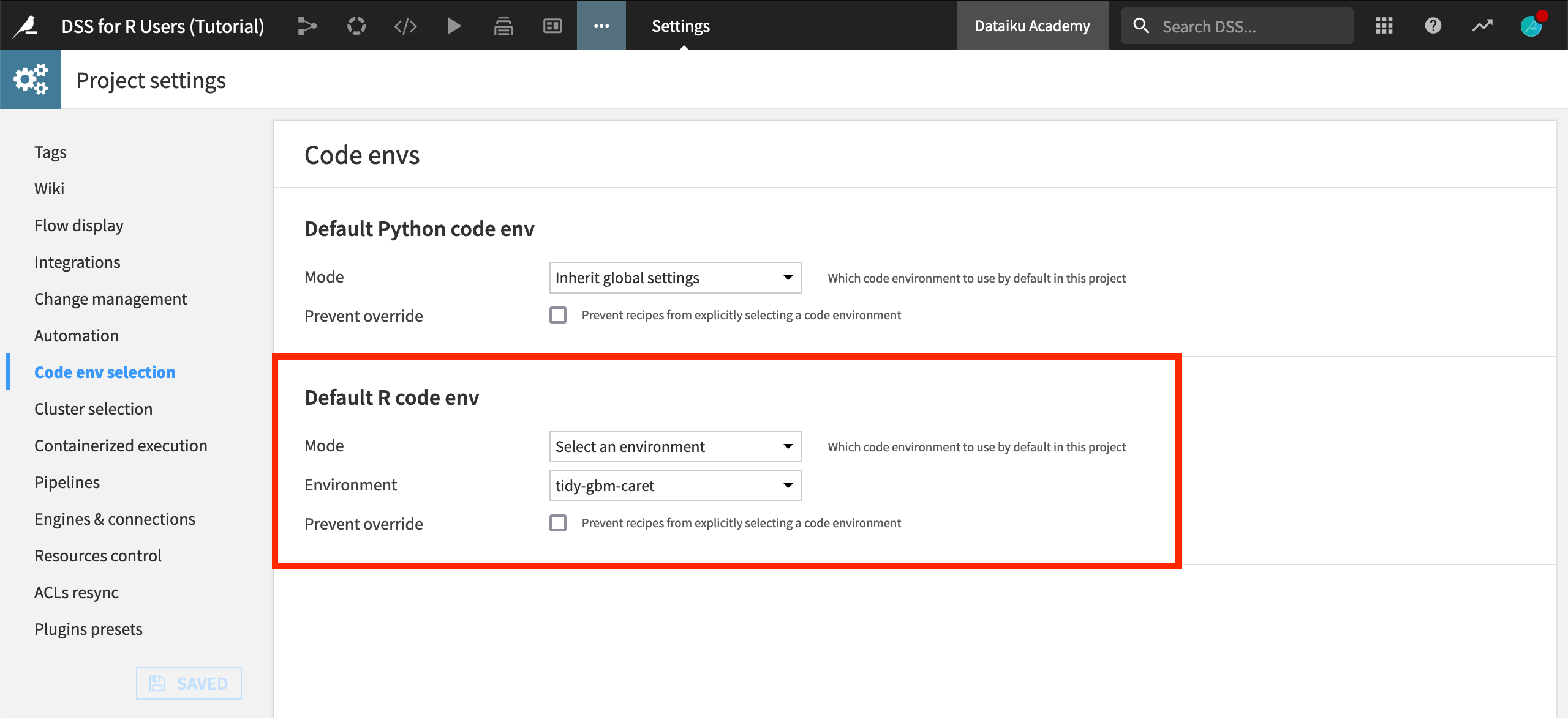
From the more options menu in the top navigation bar, choose Settings > Code env selection.
Change the Mode to Select an environment and the name of the environment that includes these four packages, in this case, “tidy-gbm-caret”.
Click Save.
With this code environment set as the project default, new R notebooks and recipes will inherit this environment, and be able to load these additional packages.
Use the R API Outside Dataiku DSS
You have seen how the DSS R API works in notebooks and recipes within Dataiku DSS. However, you can also use the same R API outside of Dataiku DSS, such as in an IDE like RStudio.
The instructions for downloading the dataiku package and setting up the connection with Dataiku DSS are covered in the product documentation. If you’d rather not set this up at this time, feel free to create a new R notebook within DSS for this section.
After configuring a connection, you can use the DSS R API to read datasets found in Dataiku DSS projects and code freely, even sharing visualizations, for example, back to the DSS instance.
In a new R script (or a new R notebook if staying within Dataiku DSS), copy/paste and run the code below to save a ggplot object as a static insight.
Note
If working outside Dataiku DSS, you’ll need to supply an API key. One way to find this is by going to Profile & Settings > API keys. Also, be sure to check that your project key is the same as given below.
library(dataiku)
library(dplyr)
library(tidyr)
library(ggplot2)

# These lines are unnecessary if running within DSS
dkuSetRemoteDSS("http(s)://DSS_HOST:DSS_PORT/", "Your API Key")
dkuSetCurrentProjectKey("DKU_TUT_R_USERS") # Replace with your project key if different

# Read the dataset as a R dataframe in memory
df <- dkuReadDataset("churn_prepared_r", samplingMethod="head", nbRows=100000)

# Create the visualization
df %>%
    select(-c(State, Area_Code, Intl_Plan, VMail_Plan)) %>%
    gather("metric", "value", -Churn) %>%
    ggplot(aes(x = value, color = Churn)) +
    facet_wrap(~ metric, scales = "free") +
    geom_density()

# Save visualization above as a static insight
dkuSaveGgplotInsight("density-plots-by-churn")
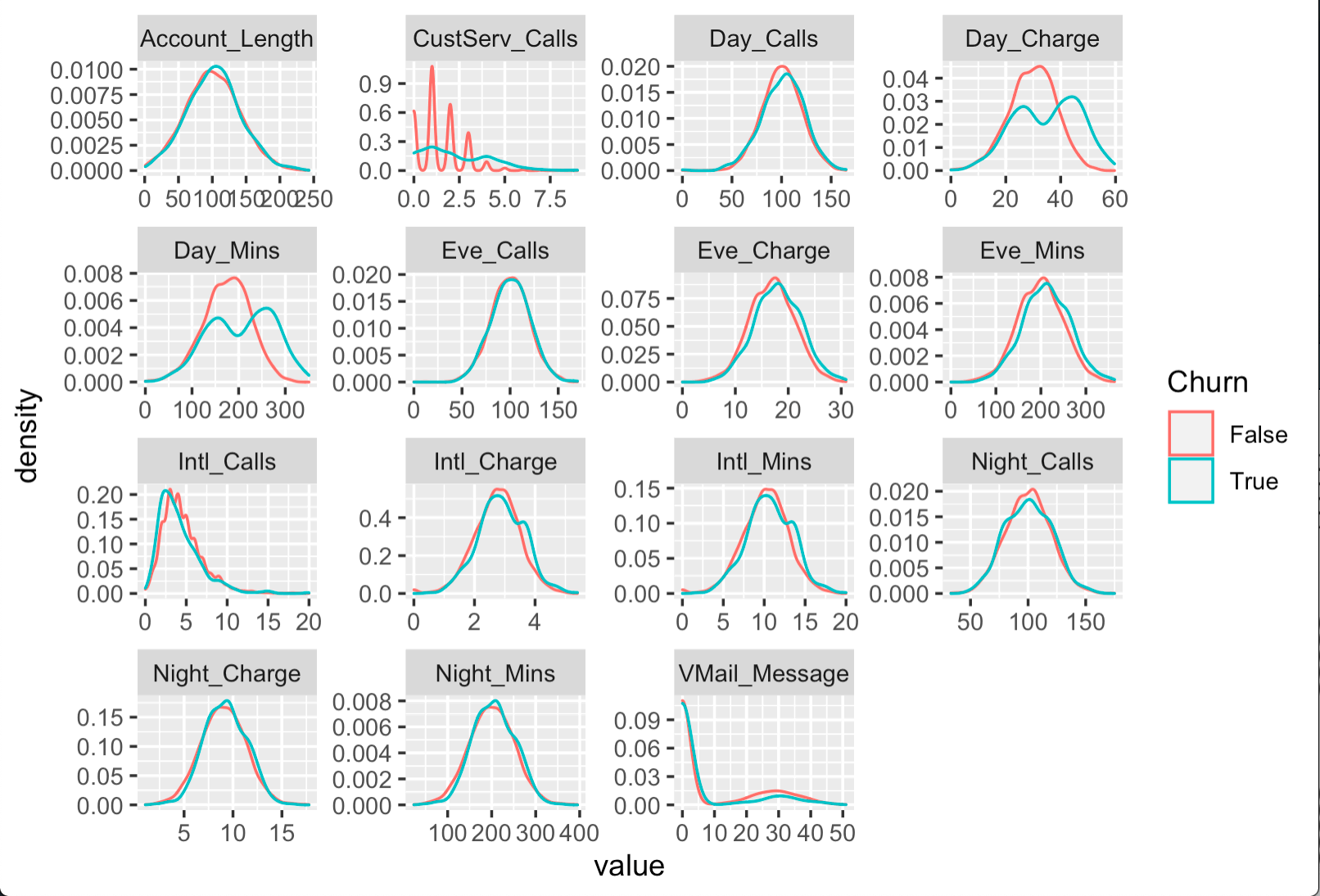
After running the code above, return to Dataiku DSS, and navigate to the Insights page (G+I) to confirm the insight has been added.
If you wish, you can publish it to a dashboard like any other insight such as native charts or model reports.
The code above visualizes the distribution for all numeric variables in the dataset among churning and returning customers. While the distribution for many variables is quite similar, a few variables like CustServ_Calls, Day_Charge, and Day_Mins follow different patterns.
Tip
In addition to ggplot2, the DSS R API has similar convenience functions for creating static insights with dygraphs, ggvis, and googleVis. You can also find more general information about static insights in the Visualization Academy course.
Edit Recipes from RStudio
Returning to the Flow, you can see that the Split recipe divides the prepared data into a training set (70%) and a test set (30%). Let’s achieve the same outcome with another R recipe, but demonstrate using the RStudio Desktop integration for editing and saving existing recipes.
Select the churn_prepared_r dataset, and add a new R recipe.
Add two output datasets,
train_randtest_r, and click Create Recipe.In the recipe editor, click Save.
Now that you have created the recipe, let’s edit it in RStudio, and save the new version back to the Dataiku DSS instance. If you followed the setup in the section above, there are no additional configuration steps needed. Alternatively, you can also skip this step, and directly edit the R recipe within DSS.
Within RStudio, create a new R script.
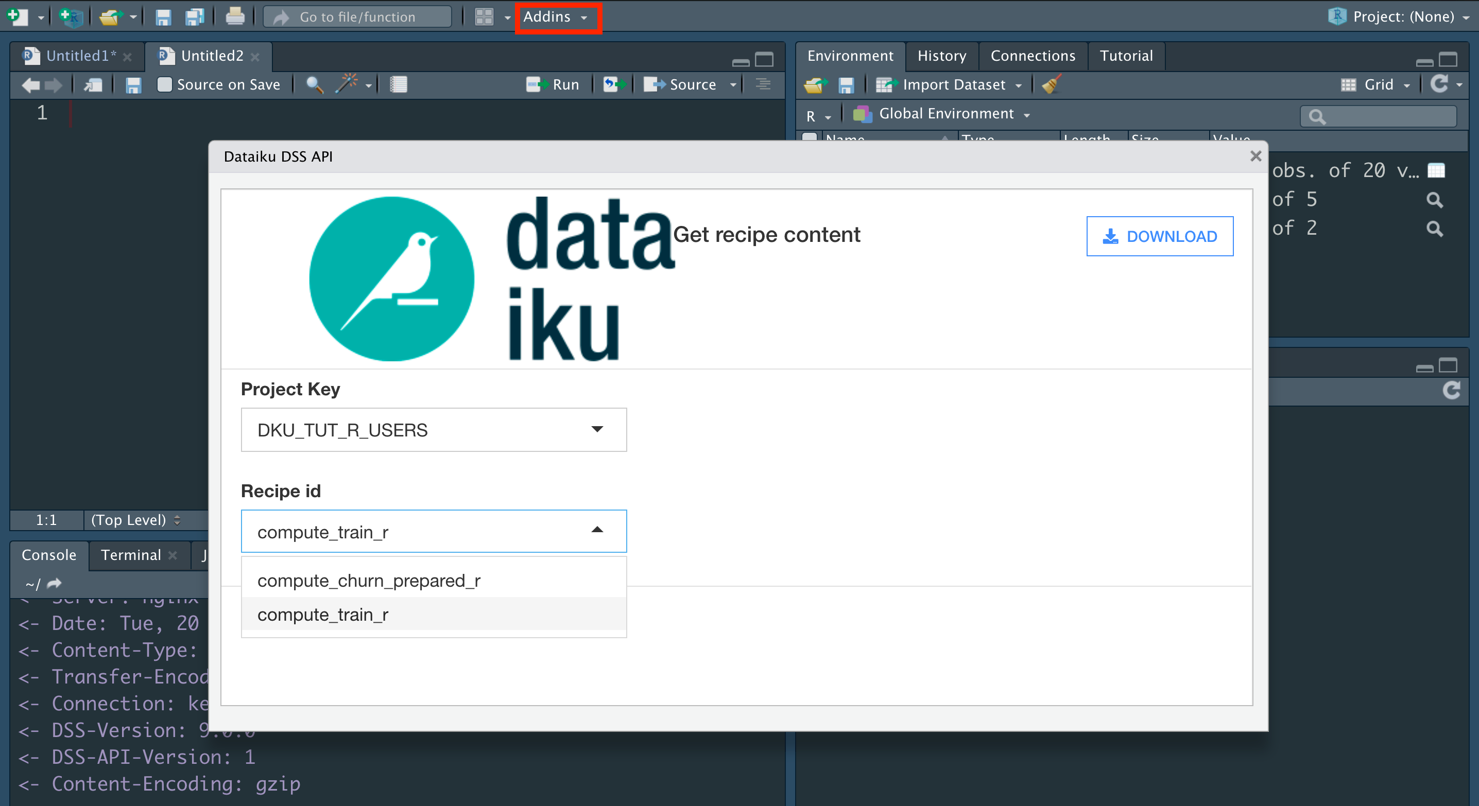
From the Addins menu, select “Dataiku: download R recipe code”.
Choose the project key, DKU_TUT_R_USERS.
Choose the Recipe ID, compute_train_r.
Click Download.
The previously empty R script should now be filled with the same R code found on the DSS instance. Let’s edit it to mimic the action of the visual Split recipe.
Replace the existing R script with the new code below.
library(dataiku)
library(dplyr)

# Recipe inputs
churn_prepared_r <- dkuReadDataset("churn_prepared_r", samplingMethod="head", nbRows=100000)

# Data preparation
churn_prepared_r %>%
    rowwise() %>%
    mutate(splitter = runif(1)) %>%
    ungroup() ->
    df_to_split

# Compute recipe outputs
train_r <- subset(df_to_split, df_to_split$splitter <= 0.7)
test_r <- subset(df_to_split, df_to_split$splitter > 0.7)

# Recipe outputs
dkuWriteDataset(train_r,"train_r")
dkuWriteDataset(test_r,"test_r")
Now, let’s save it back to the Dataiku DSS instance.
From the Addin menu of RStudio, select “Dataiku: save R recipe code”.
After ensuring the correct project key and recipe ID are selected, click Send to DSS.
Return to the DSS instance, and confirm that the new recipe has been updated after refreshing the page.
From the recipe editor, click Run to build the train_r and test_r datasets.
Note
One limitation to using the DSS R API outside DSS is the ability to write datasets. You cannot write from RStudio to a Dataiku DSS dataset as explained in this work environment tutorial.
Use Project Variables
We now have train and test sets ready for modeling, but first let’s demonstrate how project variables can be useful in a data pipeline such as this.
In the modeling stage ahead, it will be convenient to have our target variable, numeric variables, and character variables stored as separate vectors. It could be helpful to save these vectors as project variables instead of copying and pasting them for the forthcoming training and scoring recipes.
Here we are setting these variables using the DSS R API, but in many cases it’s helpful to do so manually through the UI (More options menu > Variables).
Return to the first R recipe that creates the churn_prepared_r dataset.
Click Edit in Notebook.
Add the code snippet below to the end of the recipe in new cells. Walk through it line by line to understand how this section gets and sets project variables using the functions
dkuGetProjectVariables()anddkuSetProjectVariables()from the R API.
# Empty any existing project variables
var <- dkuGetProjectVariables()
var$standard <- list(standard=NULL)
dkuSetProjectVariables(var)

# Define target, categoric, and numeric variables
target_var <- "Churn"
categoric_vars <- names(churn_prepared_r)[sapply(churn_prepared_r, is.character)]
categoric_vars <- categoric_vars[!categoric_vars %in% c("Churn")]
numeric_vars <- names(churn_prepared_r)[sapply(churn_prepared_r, is.numeric)]

# Get and set project variables
var <- dkuGetProjectVariables()

var$standard$target_var <- target_var
var$standard$categoric_vars <- categoric_vars
var$standard$numeric_vars <- numeric_vars

dkuSetProjectVariables(var)
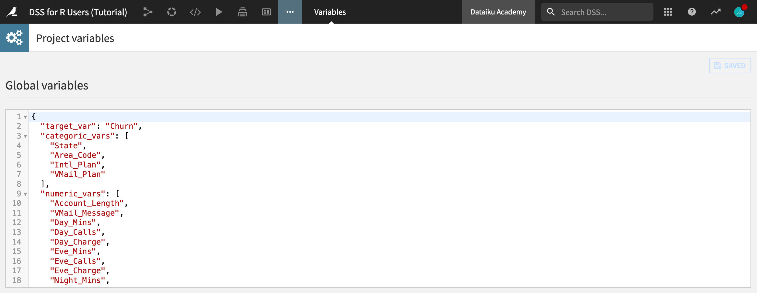
After saving back to the recipe and running it, navigate to the Variables page (More options menu > Variables) from the top navigation bar. You should see three global variables–meaning these variables are accessible anywhere in the project.
Tip
Try opening a new R notebook, and running vars <- dkuGetProjectVariables() to confirm how these variables are now accessible anywhere in the project as an R list.
For a greater conceptual understanding of project variables, as well as examples in Python, you can refer to the Academy course on Variables for Coders.
Training Machine Learning Models in R
Now that we have prepared and split the dataset, we are ready to begin modeling. The green icons in the Flow demonstrate how the visual ML interface can be used to create a machine learning model from training data, and then apply it to testing data.
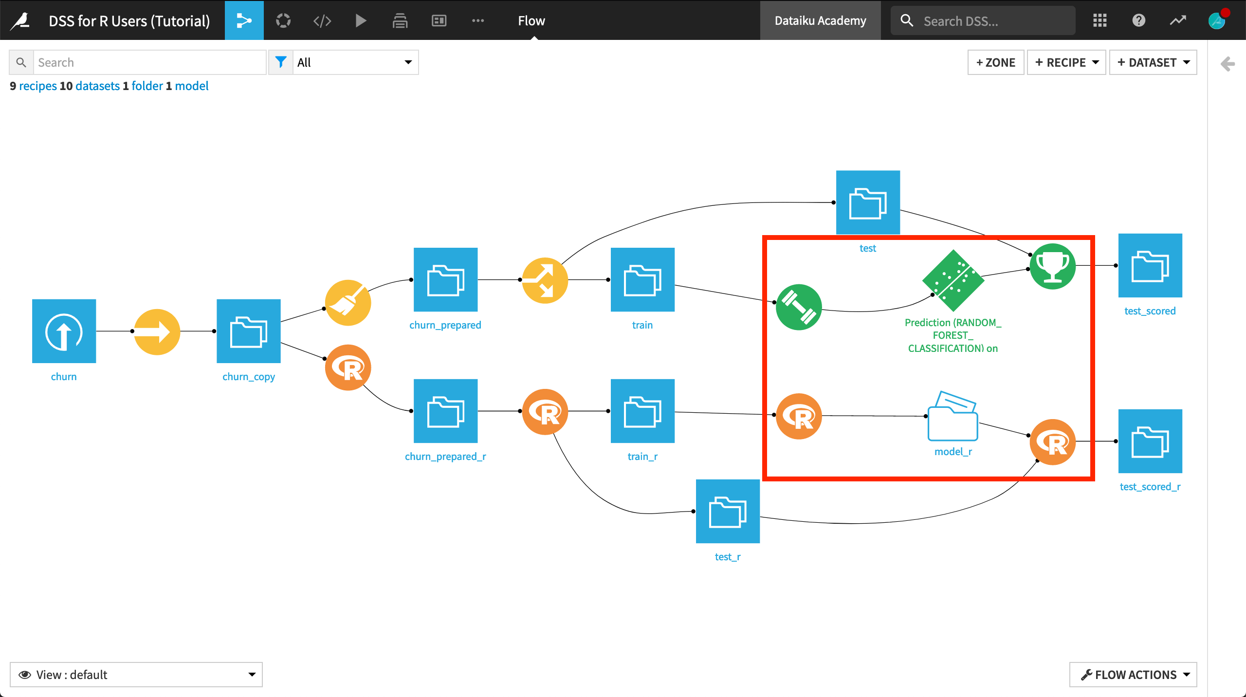
The most common workflow to achieve the same in R is similar:
First, write an R recipe that trains a model and outputs it to a managed folder.
Then, write another R recipe to score the testing data using that model.
To do this, you’ll need to be able to use the R API to interact with managed folders.
Use a Managed Folder
Given that we have the necessary packages available in the project code environment, we are ready to create an R recipe that trains a model. Unlike previous recipes however, the output of this recipe will be a managed folder instead of a dataset.
We can store any kind of file (supported or unsupported) in a managed folder, and use the DSS R API to interact with the files stored inside.
Return to the Flow, and select the train_r dataset.
Initiate a new R recipe.
Click +Add > New Folder. Name it
model_r.Click Create Folder and Create Recipe.
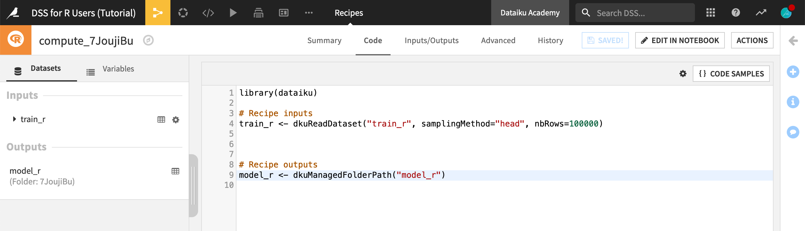
We now have the default R recipe for a dataset input and a managed folder output. Instead of using the randomly generated folder reference in the code, you can also use the folder name.
Replace the randomly-generated alphanumeric argument to
dkuManagedFolderPath()with"model_r", the name of the output folder.Click Save.
Tip
For a more conceptual look at managed folders, as well as examples in Python, register for the Academy course on Managed Folders.
Reuse R Code from a Git Repository
We now have the correct code environment, input, and output to build our model. Let’s start coding!
Imagine, however, that we want to reuse some code already developed outside of Dataiku DSS. Perhaps we want to reuse the same parameters or hyperparameter settings found in models elsewhere.
Let’s import code from a git repository into our project library so it can be used in the current recipe.
From the code menu of the top navigation bar, select Libraries, or use the shortcut G+L.
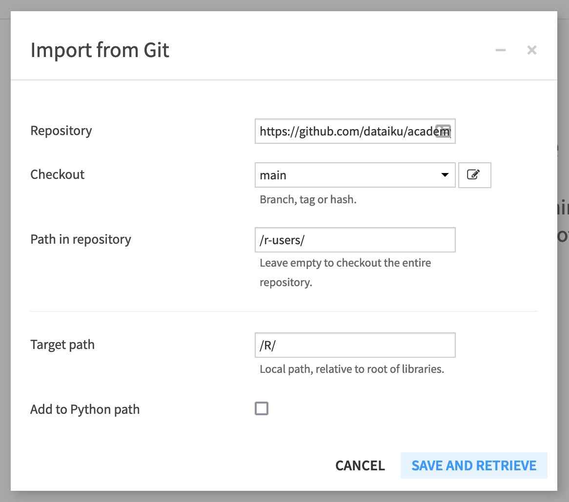
Click Git > Import from Git.
In the dialog window, supply the HTTPS link for the Repository found on GitHub (found by clicking on the Code button and then the clipboard).
Check out the “main” branch.
Add
/r-users/as the path in the repository.Add
/R/as the target path of the project library.Uncheck “Add to Python path”.
Click Save and Retrieve.
Click OK to confirm the creation of the git reference has succeeded.
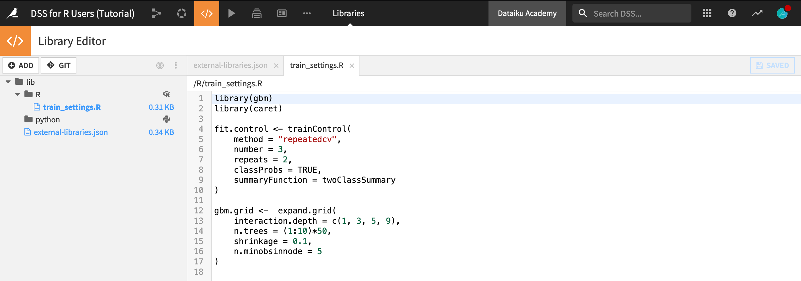
Let’s recap what this achieved:
The same file train_settings.R found in the GitHub repository is now also in the project library. It can be used in this project (or potentially in other Dataiku DSS projects as well by editing the “importLibrariesFromProjects” name of the
external-libraries.jsonfile).Open the file
external-libraries.jsonto view the git reference.
Note
The product documentation provides more details on reusing R code.
Once the git reference is created, we can import the contents of a file found in the project library into an R recipe, notebook, or webapp with the function dkuSourceLibR().
Return to the R recipe that outputs the model_r folder.
Replace the existing recipe with the code snippet below, taking note of the following:
The gbm and caret packages can be used because of the new code environment;
dkuSourceLibR()imports the objects “fit.control” and “gbm.grid” found in the “train_settings.R” file;dkuGetProjectVariables()calls the name of the target variable, as well as the set of numeric and categorical features.
library(dataiku)
library(gbm)
library(caret)

# Import from project library
dkuSourceLibR("train_settings.R")

# Recipe inputs
df <- dkuReadDataset("train_r")

# Call project variables
vars <- dkuGetProjectVariables()
target.variable <- vars$standard$target_var
features.cat <- unlist(vars$standard$categoric_vars)
features.num <- unlist(vars$standard$numeric_vars)

# Preprocessing
df[features.cat]    <- lapply(df[features.cat], as.factor)
df[features.num]    <- lapply(df[features.num], as.double)
df[target.variable] <- lapply(df[target.variable], as.factor)
train.ml <- df[c(features.cat, features.num, target.variable)]

# Training (fit.control and gbm.grid found in train_settings.R)
gbm.fit <- train(
    Churn ~ .,
    data = train.ml,
    method = "gbm",
    trControl = fit.control,
    tuneGrid = gbm.grid,
    metric = "ROC",
    verbose = FALSE
)

# Recipe outputs (local folder only)
model_r <- dkuManagedFolderPath("model_r")
setwd(model_r)
system("rm -rf *")
path <- paste(model_r, 'model.RData', sep="/")
save(gbm.fit, file = path)
Once you understand this code, run the recipe, and observe the “model.RData” file found in the output folder.
Tip
For a conceptual look at sharing code in Dataiku DSS, along with examples in Python, please register for the Academy course on Shared Code.
Local vs. Non-local Folders
The code recipe above uses dkuManagedFolderPath() to retrieve the file path used to write the model to the folder output. However, this function works only for local folders.
If the data was hosted somewhere other than the local filesystem, or the code was not running on the DSS machine, this code would fail.
Let’s modify this recipe to work for a local or non-local folder using dkuManagedFolderUploadPath() instead of dkuManagedFolderPath().
Open the recipe that produces the model_r folder.
Replace the recipe outputs section with the code below.
Then run the recipe again.
# Recipe outputs (local or non-local folder)
save(gbm.fit, file= "model.RData")
connection <- file("model.RData", "rb")
dkuManagedFolderUploadPath("model_r", "model.RData", connection)
close(connection)
Score the Test Data
There’s one last step to complete this Flow!
Now that we have a trained model in a managed folder, we can use it to score the testing data with another R recipe.
From the Flow, select the model_r folder.
Initiate a new R recipe, and add the test_r dataset as a second input.
Add a new output dataset
test_scored_r, and click Create Recipe.Replace the default code with the snippet below, and then run the recipe.
Note
In addition to standard R code, note how the code below uses the DSS R API:
dkuManagedFolderDownloadPath()interacts with the contents of a (local or non-local) managed folder. The strictly local alternative usingdkuManagedFolderPath()is also provided for demonstration in comments.dkuReadDataset()anddkuWriteDataset()handle reading and writing of dataset inputs and outputs.dkuGetProjectVariables()retrieves the values of project variables.
library(dataiku)
library(gbm)
library(caret)

# Load R model (local or non-local folder)
data <- dkuManagedFolderDownloadPath("model_r", "model.RData")
load(rawConnection(data))

# Load R model (local folder only)
# model_r <- dkuManagedFolderPath("model_r")
# path <- paste(model_r, 'model.RData', sep="/")
# load(path)

# Confirm model loaded
print(gbm.fit)

# Recipe inputs
df <- dkuReadDataset("test_r")

# Call project variables
vars <- dkuGetProjectVariables()
target.variable <- vars$standard$target_var
features.cat <- unlist(vars$standard$categoric_vars)
features.num <- unlist(vars$standard$numeric_vars)

# Preprocessing
df[features.cat]    <- lapply(df[features.cat], as.factor)
df[features.num]    <- lapply(df[features.num], as.double)
df[target.variable] <- lapply(df[target.variable], as.factor)
test.ml <- df[c(features.cat, features.num, target.variable)]

# Prediction
o <- cbind(df, predict(gbm.fit, test.ml,
                    type = "prob",
                    na.action = na.pass))

# Recipe outputs
dkuWriteDataset(o, "test_scored_r")
What’s Next?
Congratulations! You’ve built an ML pipeline in Dataiku DSS entirely with R. You’ve also demonstrated how this could be done within Dataiku DSS or from an external IDE such as RStudio.
Tip
If you have not already done so, register for the Academy course on Dataiku DSS for R Users to validate your knowledge of this material.
Next, you might take this project further by sharing results in an R Markdown report, for which you can find a tutorial here.
You might also want to develop a Shiny webapp, for which you can find a tutorial in this article.
For general reference information about Dataiku DSS and R>`_, please see the product documentation.