Churn Prediction

Outline

Churn prediction is one of the most well known applications of machine learning and data science in the Customer Relationship Management (CRM) and Marketing fields. Simply put, a churner is a user or customer that stops using a company’s products or services.

Churn applications are common in several sectors:

• Subscription business companies (think internet and telephone services providers): customers that are most likely to churn at the end of their subscription are contacted by a call center and offered a discount.

• E-commerce companies (think Amazon and the like): automatic e-mails are sent to customers that haven’t bought anything for a long time, but may respond to a promotional offer.

To read more about how Dataiku’s customers fight churn, feel free to consult our Churn and Lifetime Value success stories.

In this tutorial, you will learn how to use Dataiku DSS to create your own churn prediction model, based on your customer data. More precisely, you will learn how to:

• Define churn as a data science problem (i.e. create a variable or “target” to predict)

• Create basic features that will enable you to detect churn

• Train your first model and deploy it to predict future churn

• Learn how to deal with time-dependent features and modeling, a refined concept of machine learning and data science.

Prerequisites

This is an advanced tutorial so if you are lost at some point, please refer to the documentation or to the Basics courses. We will rely a lot on a PostgreSQL database, so you will need to set up one and the proper DSS connection as well. Also, a basic knowledge of SQL is required.

Loading the data

We will work with a toy dataset emulating the data that an e-business company (and more precisely an internet market place) might have.

First, create a new project, then import the two main datasets into DSS:

• Events are a log of what happened on your website: what page users see, what product they like or purchase…

• Product is a look-up table containing a product id, and information about its category and price. Make sure to set product_id column as bigint in the schema.

As with any data science project, the first step is to explore the data. Start by opening the events dataset: it contains a user id, a timestamp, an event type, a product id and a seller id. For instance, we may want to check the distribution of the event types. From the column header, just click on Analyze:

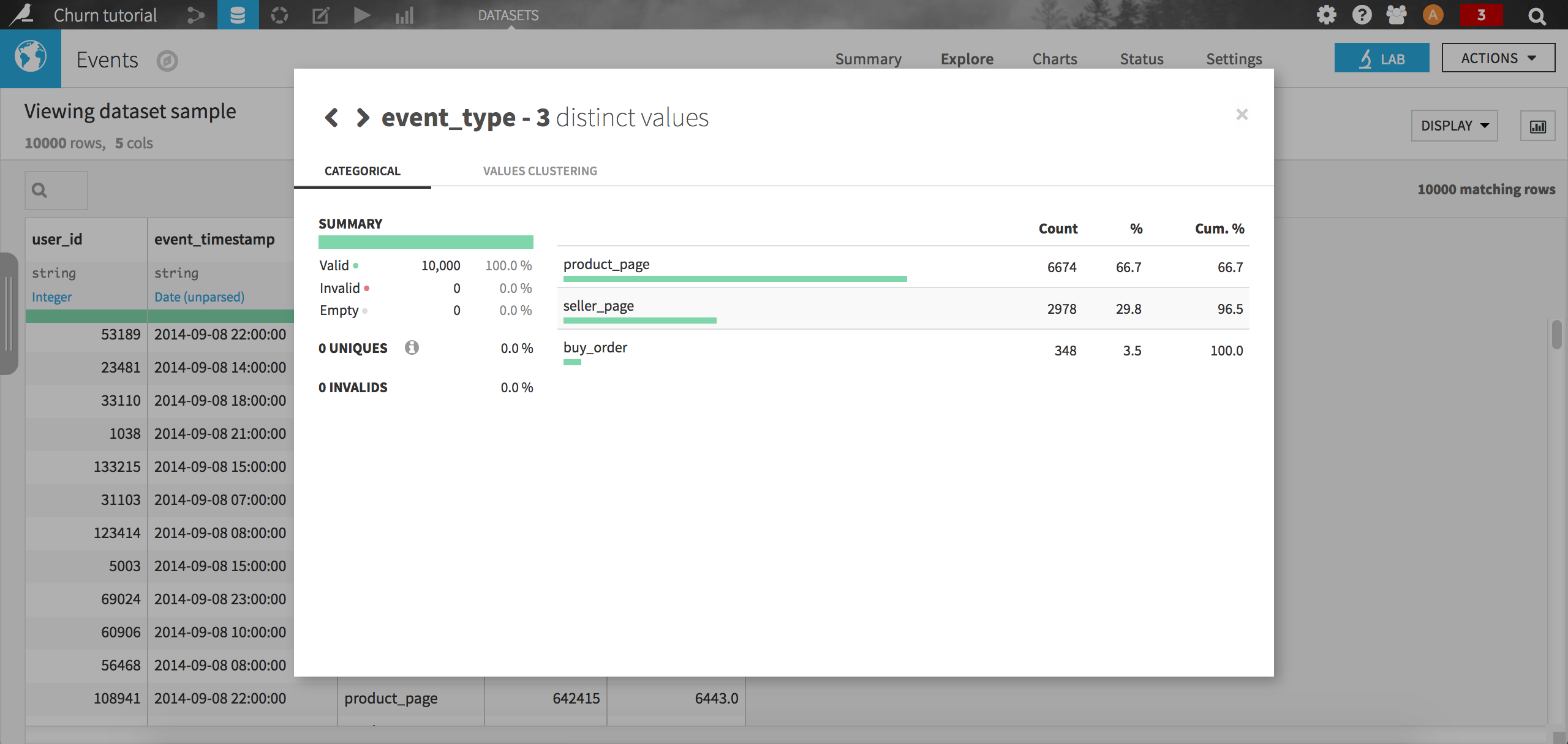
Not very surprisingly, the most common event type is viewing a product, followed by viewing a seller page (remember it is a market place e-business company). The purchase event is way less frequent with only 3.5 % of all records in the sample.

When looking at this dataset again, we can see that it contains a timestamp column which is not stored in a standard ISO format. To make it more suitable for analysis, we can quickly parse the event_timestamp column (using the format yyyy-MM-dd HH:mm:ss) using a visual data preparation script. Make sure the resulting column is stored in the Date format. Once done, you can deploy the script and directly store the resulting dataset into PostgreSQL.

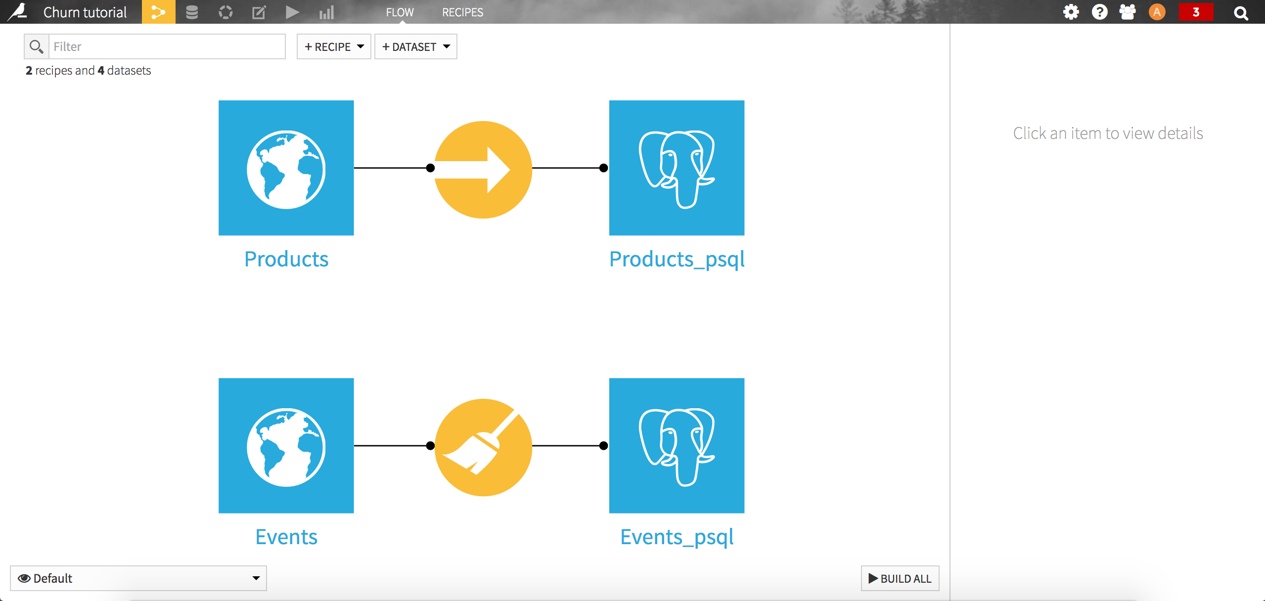
On the other hand, the product dataset contains an id, a hierarchy of categories attached to the product, and a price. You may want to check for instance the distribution of the price column, by clicking on the header and selecting Analyze in the drop-down menu. Again, load the dataset into PostgreSQL, this time using a Sync recipe.

Your flow should now look like this:

Defining the problem and creating the target

When building a churn prediction model, a critical step is to define churn for your particular problem, and determine how it can be translated into a variable that can be used in a machine learning model. The definition of churn is totally dependent on your business model and can differ widely from one company to another.

For this tutorial, we’ll use a simple definition: a churner is someone who hasn’t taken any action on the website for 4 months. We have to use a short time frame here, because our dataset contains a limited history (1 year and 3 months of data). Since many customers visit the website only once, we will focus on the “best” clients, those who generate most of the company revenue.

Our definition of churn can then be translated into the following rules:

• the target variable (i.e the one we want to model) is built by looking ahead over a 4 month period from a reference date, and flagging the customers with a “1” if they purchased a product on this time frame and “0” otherwise

• we’ll restrict our data to the customers who made at least one purchase in the previous 4 months, and total purchases at least 30 in value. This rule is to make sure we only look at the high value customers.

To create our first training dataset, we will first need to join the Products_psql and Events_psql datasets that have been synced to PostgreSQL. To do so, you can either create a new SQL recipe and write a join query yourself, or use a visual join recipe and let DSS do the work for you.

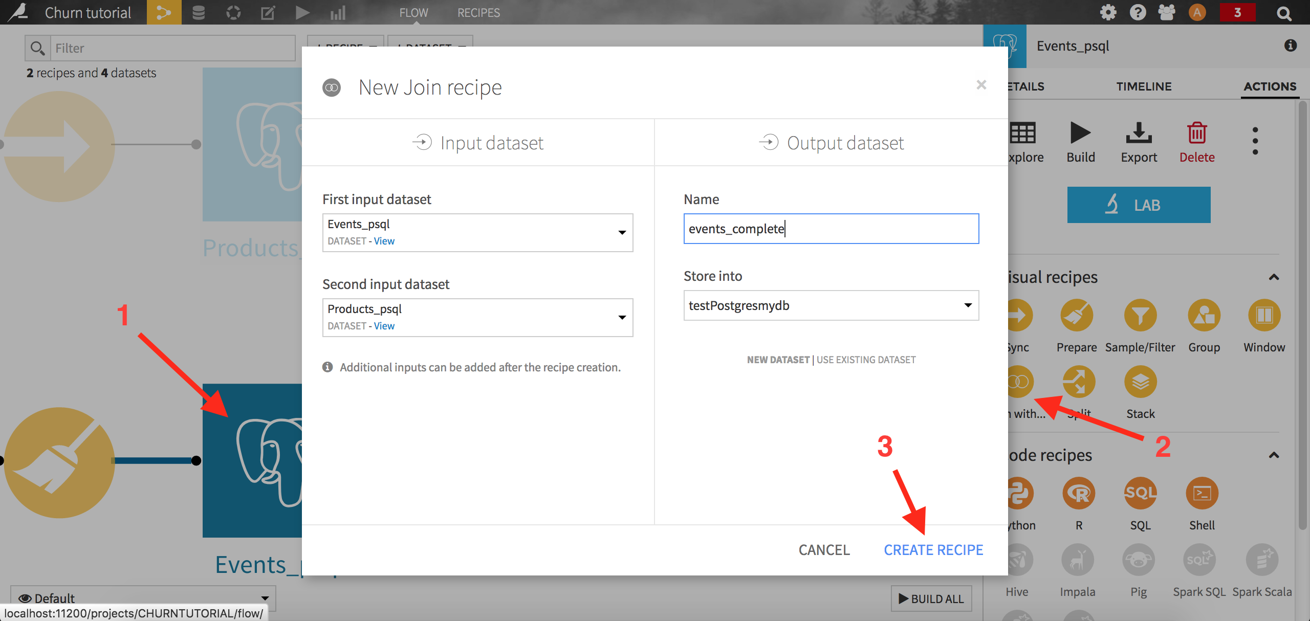
For this tutorial, we will use the visual Join recipe. From the Flow screen, left click on Events_psql. From the right panel, choose the Join with… recipe. When prompted, choose Products_sql as the second dataset, name the output events_complete, and make sure it will be written in your PostgreSQL connection again. Run the recipe.

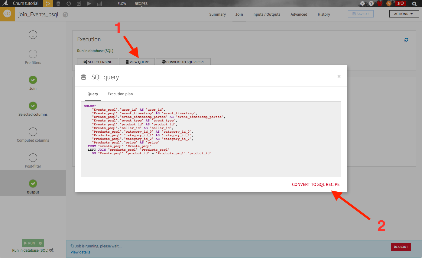
Note that you may have been able to convert the visual join recipe into an editable SQL code recipe, by navigating to the output section (from the left bar) of the recipe, clicking on View query, then Convert to SQL recipe:

We can now create our target churn variable. For the sake of the example, let’s consider 2014-08-01 as the starting point in time, the reference date. The first step is to select our “best” clients, those who bought for more than 30 dollars of products over the past 4 months. Create a SQL recipe by clicking on the “events_complete” dataset, then on the SQL icon from the right panel:

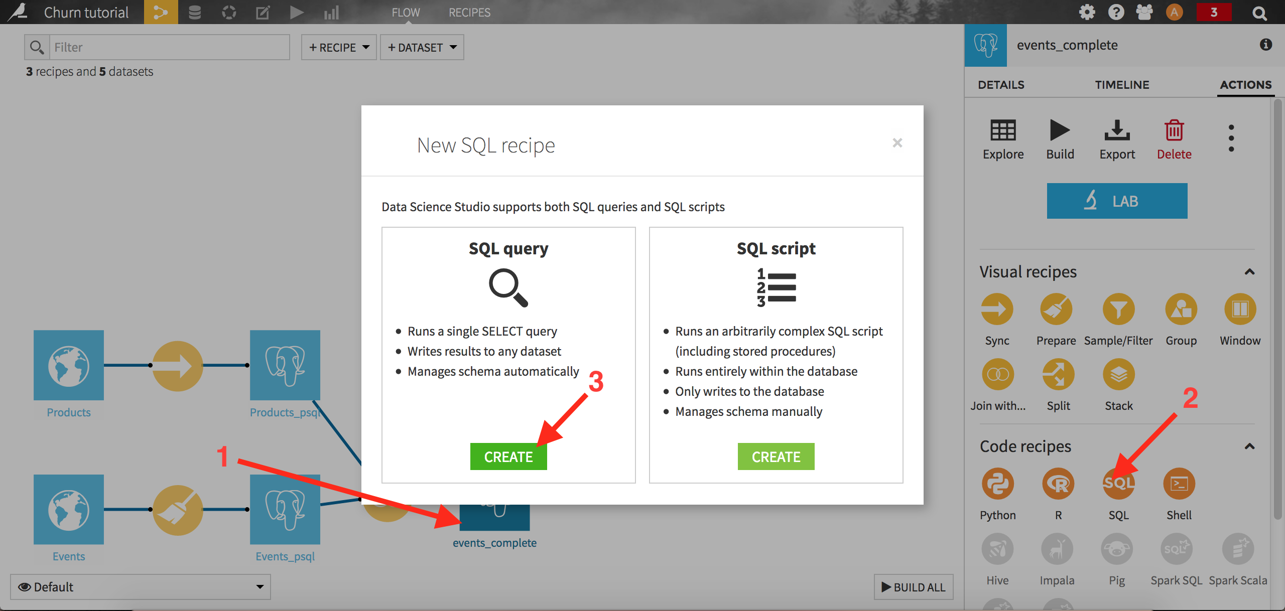
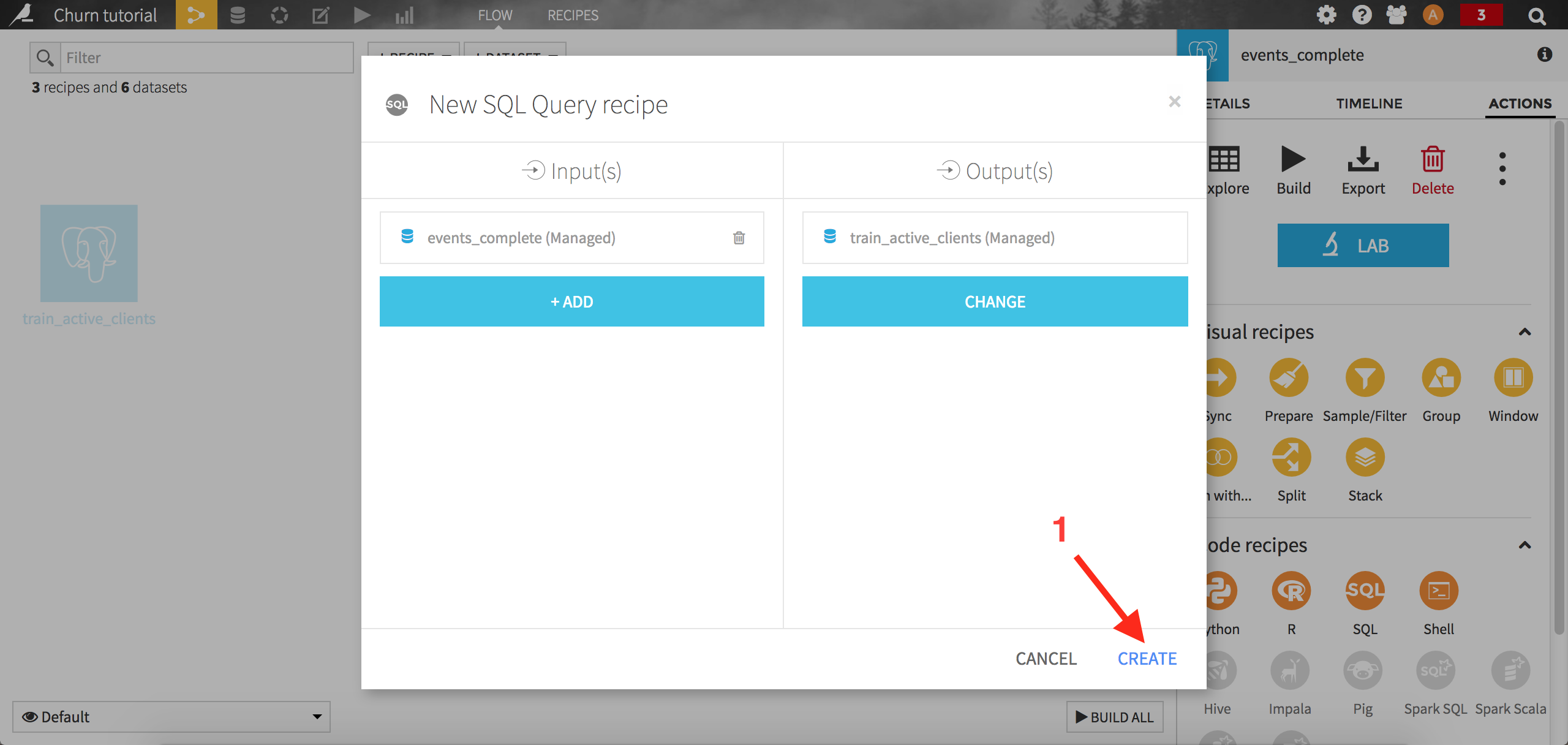
Select SQL query. DSS first asks you to create the output dataset. Name it train_active_clients and store it into your PostgreSQL connection. Click on Create to complete the creation of the recipe:

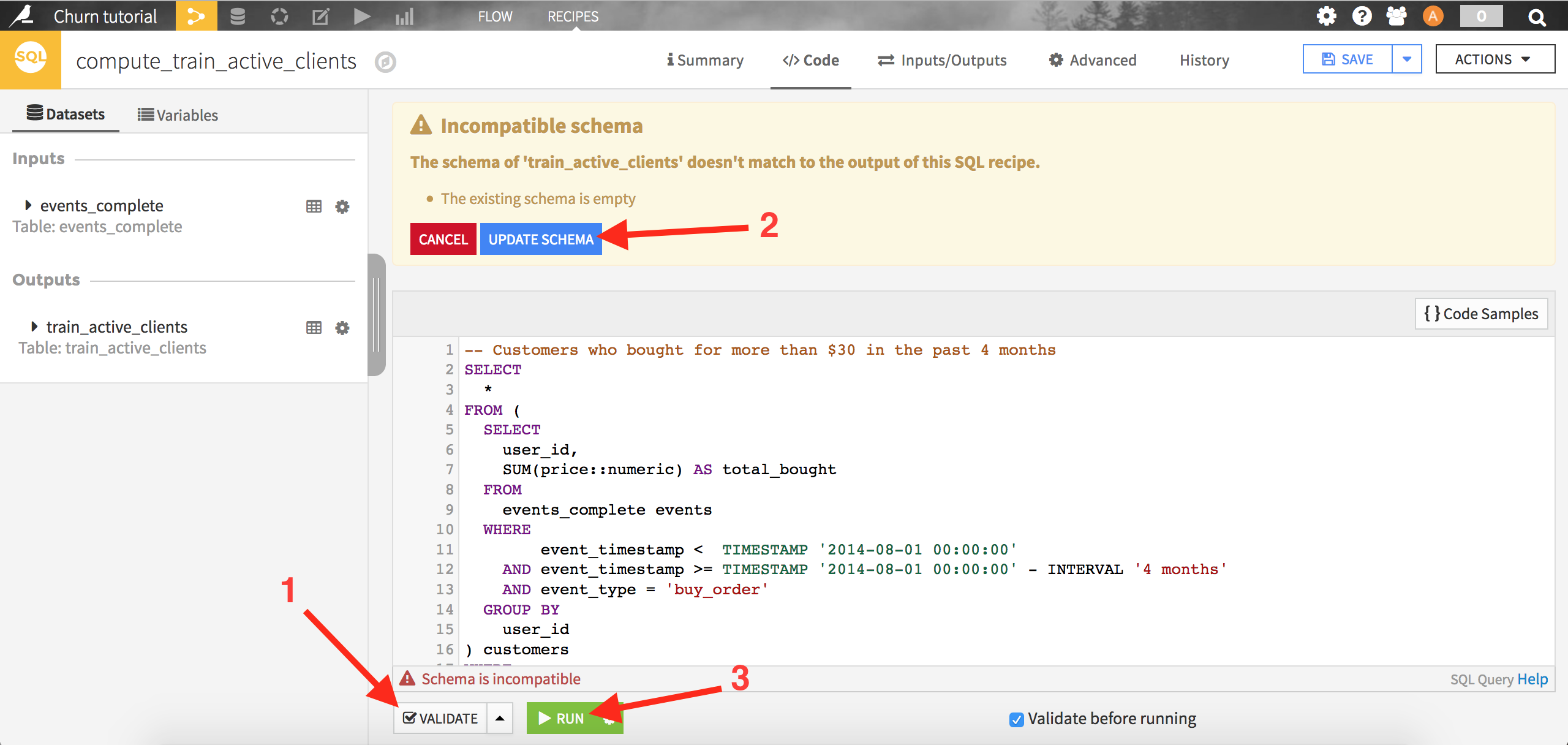
A template query is automatically generated in the code editor window. Select the best customers using the following query:

-- Customers who bought for more than $30 in the past 4 months
SELECT
  *
FROM (
  SELECT
    user_id,
    SUM(price::numeric) AS total_bought
  FROM
    events_complete events
  WHERE
        event_timestamp <  TIMESTAMP '2014-08-01 00:00:00'
    AND event_timestamp >= TIMESTAMP '2014-08-01 00:00:00' - INTERVAL '4 months'
    AND event_type = 'buy_order'
  GROUP BY
    user_id
) customers
WHERE
  total_bought >= 30

Note

Key concept: naming rules

If your PostgreSQL connection uses a Schema, Table prefix, or Table suffix, you will need to replace events_complete in this SQL with the appropriate table reference. For example, if you have the ${projectKey}_ Table prefix set and named the project “Churn Tutorial”, you need to use “CHURNTUTORIAL_events_complete” to reference the table in the SQL code.

This SQL query is the first component of our rule to identify churners: it simply filters the data on the purchase events occuring in the 4 months before our reference date, then aggregates it by customer to get their total spending over this period.

Click on Validate: DSS will ask you if you want to modify the output dataset schema, accept by clicking on Update schema. Finally, click on Run to execute the query. When the query has completed, you can click on Explore dataset train_active_clients to see the results.

The second component of our rule is to find whether or not our best customers will make a purchase in the 4 months after the reference date.

Create a new SQL recipe, where the inputs are train_active_clients (the one we just created above) and events_complete, and the output will be a SQL dataset named train. Copy the code below and run the query:

SELECT
  customer.user_id,
  CASE
    WHEN loyal.user_id IS NOT NULL THEN 1
    ELSE 0
  END as target
FROM
  train_active_clients customer
  LEFT JOIN (
    -- Users that actually bought something in the following 4 months
    SELECT distinct user_id
    FROM events_complete
    WHERE event_timestamp >= TIMESTAMP '2014-08-01 00:00:00'
      AND event_timestamp <  TIMESTAMP '2014-08-01 00:00:00' + INTERVAL '4 months'
      AND event_type = 'buy_order'
    ) loyal ON customer.user_id = loyal.user_id

The idea here is to join the previous list of “best” customers with the ones that will buy something in the next four months (found using the subquery “loyal”). The churners are actually flagged using the CASE statement: if the best customers don’t make a purchase in the next 4 months, they will not be found in the list built by the subquery, hence the NULL value. Each best customer will end up flagged with a “0” if they don’t repurchase (churner), or “1” otherwise.

This marks the end of the first big step: defining what churn is, and translating it into an actual variable that can be used by a machine learning algorithm.

Building a first model

Now that our target variable is built, we need to create the complete train set that will store a list of features as well. The features are the variables we’ll use to try to predict churn.

Let’s create a new SQL recipe, with the train and events_complete datasets as inputs, and a new SQL dataset named train_enriched as output. The recipe is made of the following code:

SELECT train.*
    , nb_products_seen
    , nb_distinct_product
    , nb_dist_0 , nb_dist_1, nb_dist_2
    , amount_bought , nb_product_bought
    , active_time
FROM train
LEFT JOIN (
    -- generate features based on past data
    SELECT user_id
        , COUNT(product_id) AS nb_products_seen
        , COUNT(distinct product_id) AS nb_distinct_product
        , COUNT(distinct category_id_0) AS nb_dist_0
        , COUNT(distinct category_id_1) AS nb_dist_1
        , COUNT(distinct category_id_2) AS nb_dist_2
        , SUM(price::numeric * (event_type = 'buy_order')::int ) AS amount_bought
        , SUM((event_type = 'buy_order')::int ) AS nb_product_bought
        , EXTRACT(
           EPOCH FROM (
            TIMESTAMP '2014-08-01 00:00:00' - MIN(event_timestamp)
           )
          )/(3600*24)
              AS active_time
    FROM events_complete
    WHERE event_timestamp < TIMESTAMP '2014-08-01 00:00:00'
    GROUP BY user_id
    ) features ON train.user_id = features.user_id

This query adds several features to the train dataset (containing the target variable). An intuition is that the more a person is active, the less likely she is to churn.

We hence create the following features for each user:

• total number of products seen or bought on website

• number of distinct product seen or bought

• number of distinct categories (to have an idea of the diversity of purchases of a user)

• total number of products bought

• and total amount spent

Once this first limited set of features is created, our training set is ready. As in the Machine Learning Basics course, create a baseline model to predict the target:

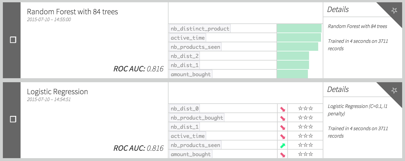
This AUC scores are not that bad for a first model. Let’s deploy it.

Deploying the model

The model being created and trained, we may now want to be able to use it to “score” potential churners on a regular basis (every month for example). To make sure the model will remain robust over time, and to replicate what is going to happen when using it (new records arrive on a regular basis), we can create the “test” set to score.

This is where the modeling process, and notably the train/test split strategy, gets a little bit more tricky.

Let’s say our current timestamp is T, then all the features created for the test set must depend on times t <= T. Since we need to keep 4 months worth of future data to create the target variable in our training set (did the customer repurchase?), the target will be generated from the data in the [T, T + 4 months] time interval, and the train features will use values in the [T - 4 months, T] interval, this way data “from the future” won’t leak in the features. Since we originally choose the reference date to be 2014-08-01, let’s choose T as 2014-12-01 for our test set to stay aligned with what we have already done. To sum up:

• train set target is based on data between 2014-08-01 and 2014-12-01

• train set features are based on data before 2014-08-01

• test set features are based on data before 2014-12-01

• test set optional target can be computed with data between 2014-12-01 and 2015-03-01

Also, to make our scripts more flexible, we will set these train and test reference dates as DSS global parameters, as described here. Click on the Administration menu on the top right of your screen, then select Settings on the top right and Variables on the top left:

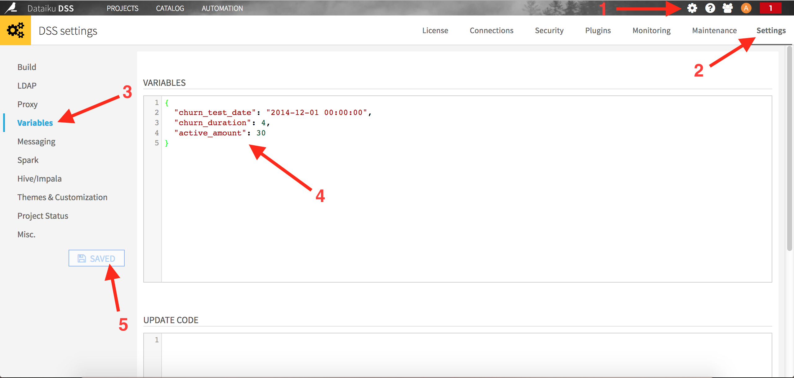
The content of the variables editor is the following:

{
  "churn_test_date": "2014-12-01 00:00:00",
  "churn_duration" : 4,
  "active_amount" : 30
}

The first parameter is our reference date, when we want to actually score our clients. In a production setting, this could be replaced by “today” for example (we refresh the churn model to predict what is going to happen everyday). The second parameter defines the number of months to use to build our features. The last parameters is the threshold we used for our “best” client definition.

Now let’s update our 3 sql recipes using these new global variables. For example the first one (selecting the customers to use for our training set) becomes:

SELECT * -- select customers with total >= active_amount
FROM (
  -- select active users and calculate total bought in the period
  SELECT
    user_id ,
    SUM(price::numeric) AS total_bought
  FROM
    events_complete events
  WHERE
        event_timestamp <  TIMESTAMP '${churn_test_date}'
                           - INTERVAL '${churn_duration} months'
    AND event_timestamp >= TIMESTAMP '${churn_test_date}'
                           - 2 * INTERVAL '${churn_duration} months'
    AND event_type = 'buy_order'
  GROUP BY
    user_id
) customers
WHERE
  total_bought >= '${active_amount}'
;

Modify the two others recipes accordingly.

Moving to the test set, you should also be able to create the 3 required datasets using these SQL recipes:

-- Test set population
SELECT
  *
FROM (
  SELECT
    user_id,
    SUM(price::numeric) AS total_bought
  FROM
    events_complete events
  WHERE event_timestamp <  TIMESTAMP '${churn_test_date}'
    AND event_timestamp >= TIMESTAMP '${churn_test_date}'
                         - INTERVAL '${churn_duration} months'
    AND event_type = 'buy_order'
  GROUP BY
    user_id
) customers
WHERE
  total_bought >= '${active_amount}'

-- Test set target variable
SELECT
  client.user_id,
  CASE
    WHEN loyal.user_id IS NULL THEN 1
    ELSE 0
  END as target
FROM
  test_active_clients client
  LEFT JOIN (
    SELECT DISTINCT user_id
    FROM events_complete
    WHERE event_timestamp >= TIMESTAMP '${churn_test_date}'
      AND event_timestamp <  TIMESTAMP '${churn_test_date}'
                           + INTERVAL '${churn_duration} months'
      AND event_type = 'buy_order'
  ) loyal ON client.user_id = loyal.user_id

-- Complete test set
SELECT
  test.*,
  nb_products_seen,
  nb_distinct_product,
  nb_dist_0,
  nb_dist_1,
  nb_dist_2,
  amount_bought,
  nb_product_bought,
  active_time
FROM
  test
  LEFT JOIN (
    SELECT
      user_id,
      COUNT(product_id) as nb_products_seen,
      COUNT(distinct product_id) as nb_distinct_product,
      COUNT(distinct category_id_0) as nb_dist_0,
      COUNT(distinct category_id_1) as nb_dist_1,
      COUNT(distinct category_id_2) as nb_dist_2,
      SUM(price::numeric * (event_type = 'buy_order')::int ) as amount_bought,
      SUM((event_type = 'buy_order')::int ) as nb_product_bought,
      EXTRACT(
       EPOCH FROM (
        TIMESTAMP '${churn_test_date}' - MIN(event_timestamp)
       )
      ) / (3600*24) as active_time
    FROM
      events_complete
    WHERE
      event_timestamp < TIMESTAMP '${churn_test_date}'
    GROUP BY
      user_id
  ) features ON test.user_id = features.user_id

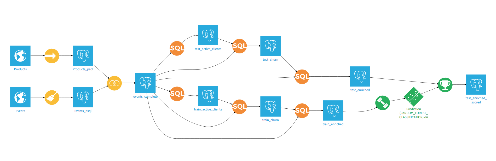
Once this is done, you just have to go back to your model and use it to score the test dataset. In the end, your DSS flow should look like this:

Even though we made great progress, we still have work to do. The major problem is that we did not take time into account to separate (by design of churn) our train and test sets, neither in the evaluation of our model, nor in the features engineering. Let’s see why this can be a big mistake.

Going deeper into churn modeling

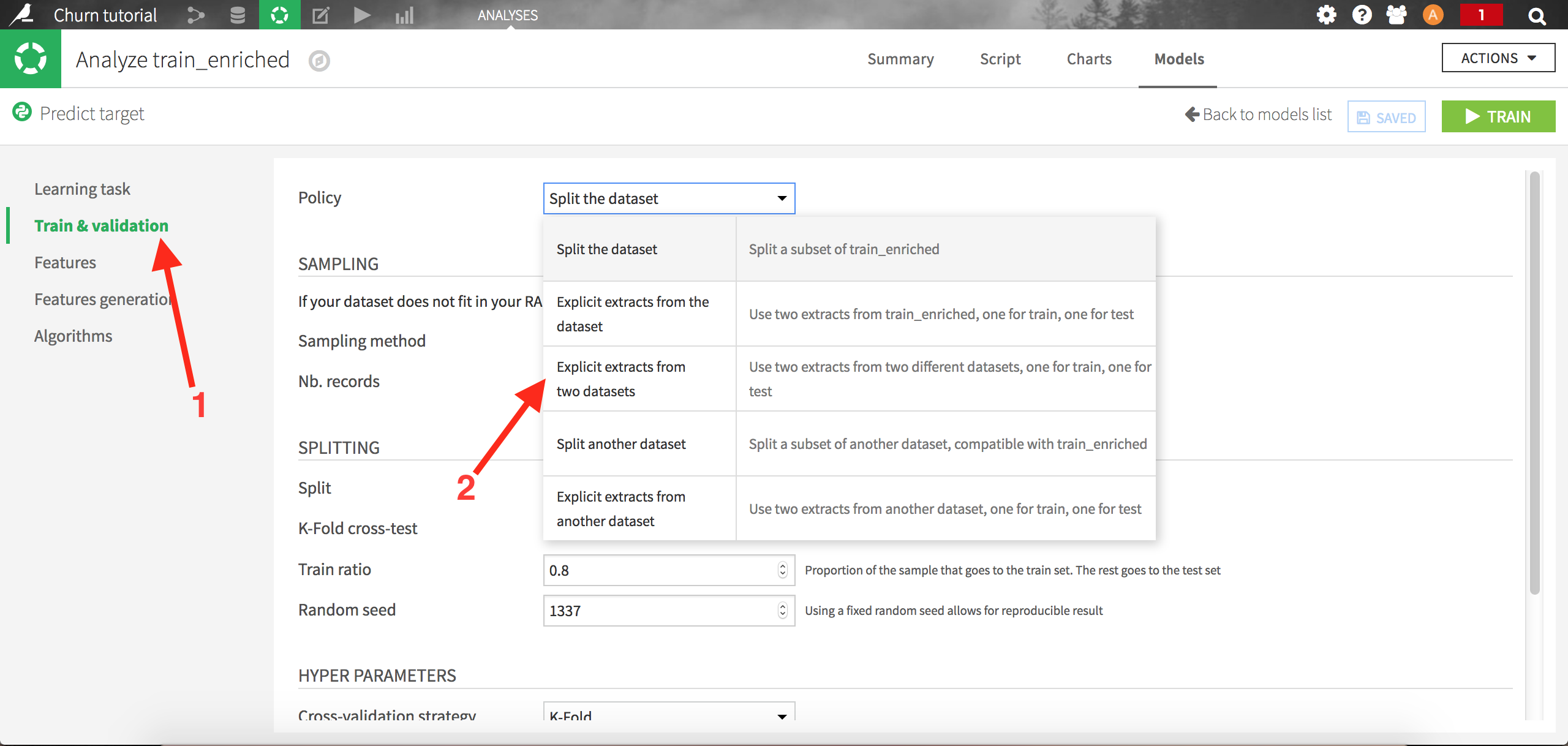
In the previous section, we generated a test set containing the target variable, we should then be able to evaluate our model on this dataset. Doing so will give us a better approximation of the real model performance, since it takes time into account. We used previously the default random 80% (train) / 20% (test) split, but this assumes that our flow and model are time-independent, an assumption clearly violated in our construction.

Let’s go back to our model, and go to the settings screens. We are going to change the Train & validation policy. Let’s choose “Explicit extracts from two datasets”:

Choose test_enriched as the Test Set and save. DSS will now train the models on the train set, and evaluate it using an auxiliary test set (test_enriched):

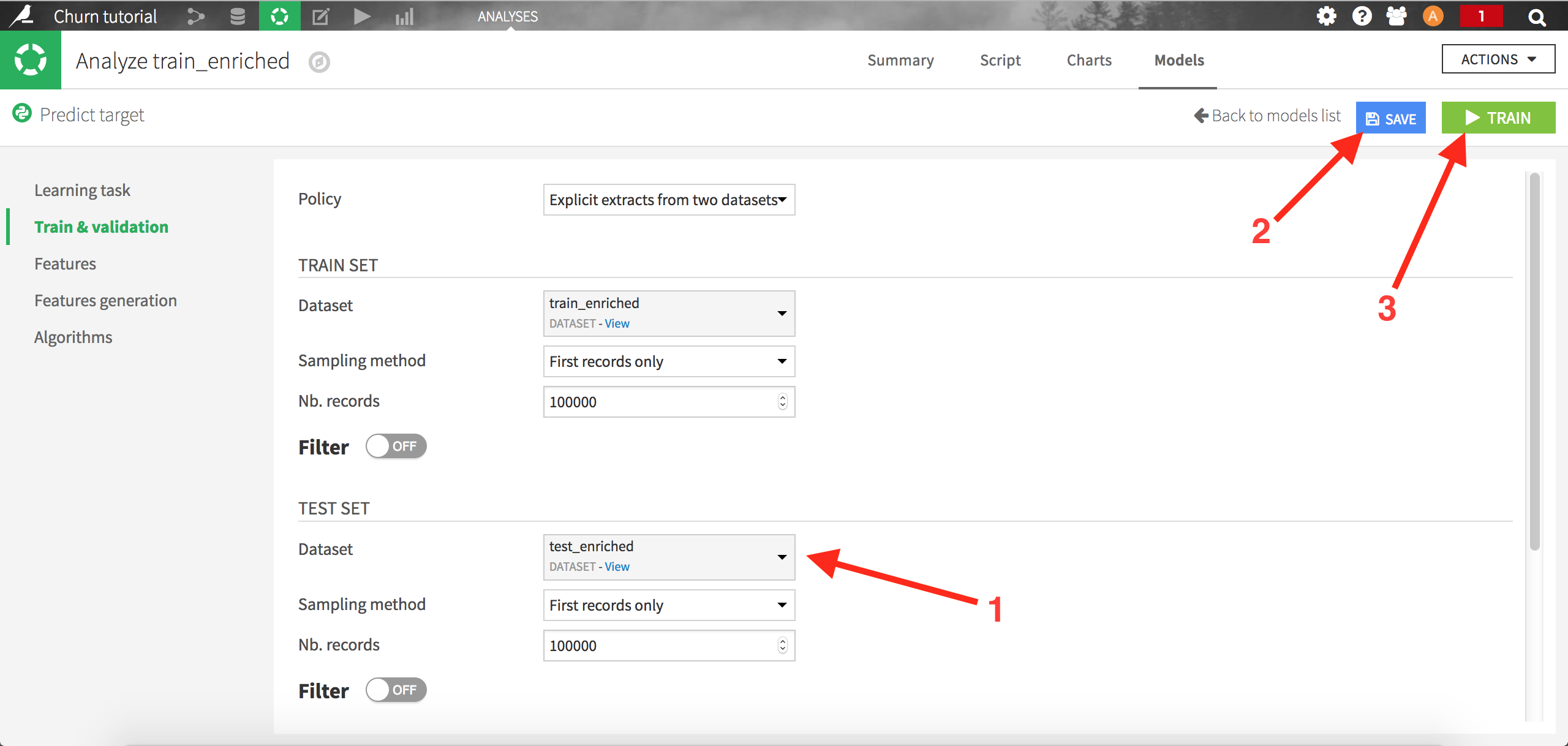
Click on “train” to start the calculations. The summary model list should now be updated with new runs:

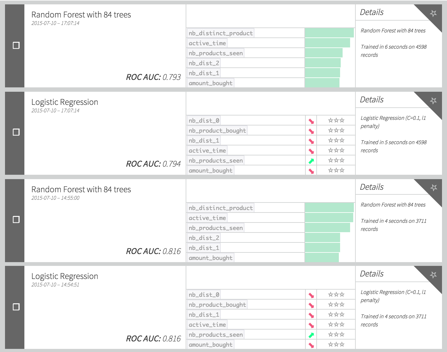
Note that the performance (here measured via the AUC) decreased a lot, even though we are using more data (because there is no train split, we have 1.25 times more data in our train set). The reason of this decrease is the combination of 2 factors:

• Things inherently change with time. The patterns observed in our train set may have changed in the test set, since this one uses fresher data. Even though this effect can be rather small, it will however always exist when dealing with time dependent data (and train/test split strategy), and this is something that needs to be taken into account when creating such models.

• Our features are poorly designed, since we created them using the whole history of data. The amount of data available to build the features increases over time: here the test set would rely on a much longer history than the train set (because the train set uses “older” data), so our features distributions would differ a lot between the train set and the test set.

This issue can be solved by designing smarter features, like count of product seen in the past “k” weeks from the reference date, or by creating ratios such as the total amount spent divided by total duration of user activity. We can then transform the code used to generate the train_enriched dataset this way:

SELECT
  -- Basic features
  basic.*,
  -- "Trend" features
  one.nb_products_seen::numeric / basic.nb_products_seen AS rap_nb_products_seen ,
  one.nb_distinct_product::numeric / basic.nb_distinct_product AS rap_nb_distinct_product,
  one.nb_dist_0::numeric / basic.nb_dist_0 AS rap_nb_nb_dist_0 ,
  one.nb_dist_1::numeric / basic.nb_dist_1 AS rap_nb_dist_1 ,
  one.nb_dist_2::numeric / basic.nb_dist_2 AS rap_nb_dist_2 ,
  one.nb_seller::numeric / basic.nb_seller AS rap_nb_seller ,
  one.amount_bought::numeric / basic.amount_bought AS rap_amount_bought ,
  one.nb_product_bought::numeric / basic.nb_product_bought AS rap_nb_product_bought ,
  -- global features
  glob.amount_bought / active_time AS amount_per_time ,
  glob.nb_product_bought::numeric / active_time AS nb_per_time ,
  glob.amount_bought AS glo_bought ,
  glob.nb_product_bought AS glo_nb_bought ,
  -- target
  target
FROM
  train

  LEFT JOIN (
    SELECT
      user_id,
      COUNT(product_id) AS nb_products_seen,
      COUNT(distinct product_id) AS nb_distinct_product,
      COUNT(distinct category_id_0) AS nb_dist_0,
      COUNT(distinct category_id_1) AS nb_dist_1,
      COUNT(distinct category_id_2) AS nb_dist_2,
      COUNT(distinct seller_id) AS nb_seller ,
      SUM(price::numeric * (event_type = 'buy_order')::int ) AS amount_bought,
      SUM((event_type = 'buy_order')::int ) AS nb_product_bought
    FROM
      events_complete
    WHERE
          event_timestamp <  TIMESTAMP '${churn_test_date}'
                           - INTERVAL '${churn_duration} months'
      AND event_timestamp >= TIMESTAMP '${churn_test_date}'
                           - 2 * INTERVAL '${churn_duration} months'
    GROUP BY
      user_id
  ) basic ON train.user_id = basic.user_id

  LEFT JOIN (
    SELECT
      user_id,
      COUNT(product_id) AS nb_products_seen,
      COUNT(distinct product_id) AS nb_distinct_product,
      COUNT(distinct category_id_0) AS nb_dist_0,
      COUNT(distinct category_id_1) AS nb_dist_1,
      COUNT(distinct category_id_2) AS nb_dist_2,
      COUNT(distinct seller_id) AS nb_seller,
      SUM(price::numeric * (event_type = 'buy_order')::int ) AS amount_bought,
      SUM((event_type = 'buy_order')::int ) AS nb_product_bought
    FROM
      events_complete
    WHERE
         event_timestamp <  TIMESTAMP '${churn_test_date}'
                          - INTERVAL '${churn_duration} months'
     AND event_timestamp >= TIMESTAMP '${churn_test_date}'
                          - INTERVAL '${churn_duration} months'
                          - INTERVAL '1 months'
    GROUP BY
      user_id
) one ON train.user_id = one.user_id

LEFT JOIN (
  SELECT
    user_id,
    SUM(price::numeric * (event_type = 'buy_order')::int ) AS amount_bought,
    SUM((event_type = 'buy_order')::int ) AS nb_product_bought,
    EXTRACT(
     EPOCH FROM (
        TIMESTAMP '${churn_test_date}'
      - INTERVAL '${churn_duration} months'
      - MIN(event_timestamp)
     )
    ) / (3600*24) AS active_time
  FROM
    events_complete
  WHERE
    event_timestamp < TIMESTAMP '${churn_test_date}'
                    - INTERVAL '${churn_duration} months'
  GROUP BY
    user_id
) glob ON train.user_id = glob.user_id

This SQL recipe looks rather cumbersome, but if we look at it more in details, we see that we generated three kinds of variables:

• “basic” features, which are the exact same counts and sums as in the previous section, except that they are now based only on the previous rolling month. This way, our variables are less dependent on time.

• “trend” variables, which are the ratio between the features calculated on one rolling week, and those calculated on one rolling month. With these variables, we intend to capture if the consumer has been recently increasing or decreasing its activity.

• “global” features, which capture the information on the whole customer life. These variables are rescaled by the total lifetime of the customer so as to be less correlated with time.

By adapting in the same way the test_enriched dataset (modifying table names and dates in the query), you should be able to retrain your model, and have performances similar to this:

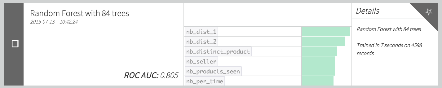
We managed to improve our performance by more than 0.01 point of AUC, doing some fairly basic feature engineering.

Wrap-up

Congratulations if you made it until the end :) This tutorial was rather long and technical, but gives you an idea about how complex this could get to create a churn model. We saw some of the major difficulties:

• defining properly what is churn and how to translate it into a “target” variable

• creating features depending on time, and relatively to a reference date

• choosing the proper cross-validation strategy

Of course, handling this kind of models in real life will take you much further. It is very frequent to include hundreds of features, or even spend a few days trying to properly scope the churn definition.

And this might only be a first step. Indeed, you’ll probably want to model the propensity to respond to different kind of anti-churn offers, or model the true incremental effect of these systems (“lift modeling”).