Data Scientist Quick Start

Getting Started

Dataiku is a collaborative, end-to-end data science and machine learning platform that unites data analysts, data scientists, data engineers, architects, and business users in a common space to bring faster business insights.

In this quick start, you will learn about the ways that Dataiku DSS can provide value to coders and data scientists through a simple use case: predicting whether a customer will generate high or low revenue. You’ll explore an existing project and improve upon the steps that a data analyst team member already performed. Some of the tasks you’ll perform include:

• exploring data using a Python notebook;

• engineering features using code in a notebook and code recipe;

• training a machine learning model and generating predictions;

• monitoring model performance using a scenario, and more.

This hands-on tutorial is designed for coders and data scientists entirely new to Dataiku DSS. Because Dataiku DSS is an inclusive enterprise AI platform, you’ll see how many actions performed using the coding interface can be completed using the point-and-click interface.

Note

This tutorial is part of our quick start program that includes:

• AI Consumer which explores the visual interface,

• Business Analyst which covers data pipelines and advanced analytics,

• Data Engineer which focuses on collaboration, model metrics, and Flow improvement, and

• Data Scientist which covers the use of the coding interface in Dataiku DSS.

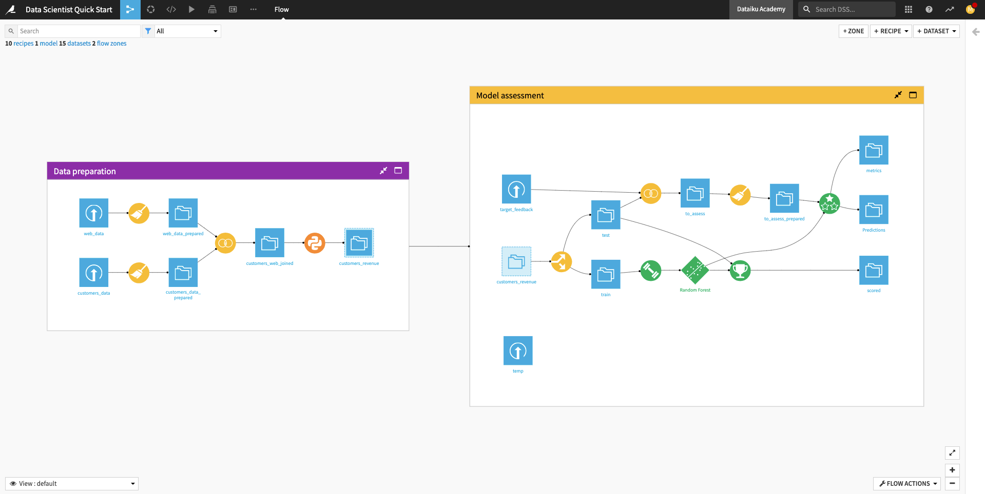
When you’re finished, you will have built the workflow below and understood all of its components!

Prerequisites

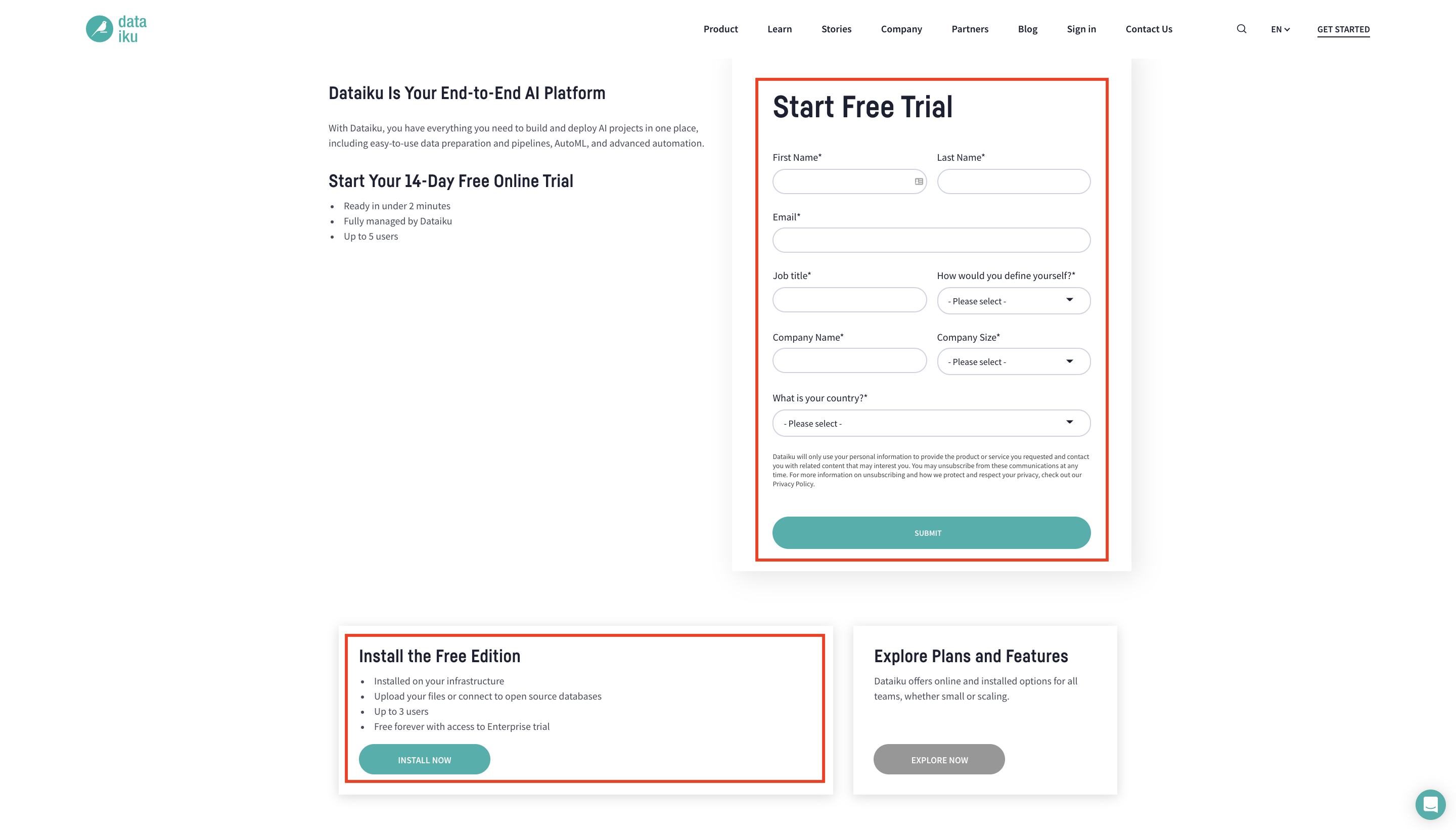
To follow along or reproduce the tutorial steps, you will need access to an instance of Dataiku DSS (version 9.0 or above). If you do not already have access, you can get started in one of two ways:

• Start a 14-Day Free Online Trial, or

• Download the free edition.

Tip

For each section of this quick start, written instructions are recorded in bullet points. Be sure to follow these while using the screenshots as a guide. We also suggest that you keep these instructions open in one tab of your browser and your Dataiku DSS instance open in another.

You can find a read-only completed version of the final project in the public gallery.

Create the Project

When you open your instance of Dataiku DSS, you’ll immediately land on the Dataiku homepage. Here, you’ll be able to browse projects, recent items, dashboards, and applications that have been shared with you.

Note

A Dataiku DSS project is a holder for all work on a particular activity.

You can create a new project in a few different ways. You can start a blank project or import a zip file. You might also have projects already shared with you based on the user groups to which you belong.

We’ll create our project from an existing Dataiku tutorial project.

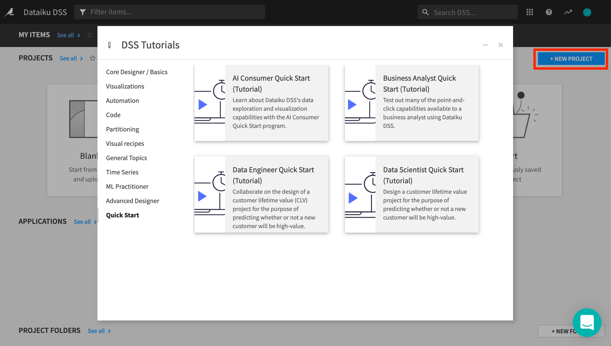
• From the Dataiku DSS homepage, click on +New Project.

• Choose DSS Tutorials > Quick Start > Data Scientist Quick Start (Tutorial).

• Click OK when the tutorial has been successfully created.

Note

You can also download the starter project from this website and import it as a zip file.

Explore the Project

After creating the project, you’ll land on the project homepage. This page contains a high-level overview of the project’s status and recent activity, along with shortcuts such as those found in the top navigation bar.

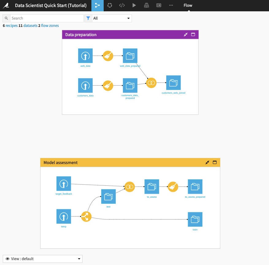
• From the top navigation bar, click the Flow icon to open up the project workflow, called the Flow.

Note

The Flow is the visual representation of how data, recipes (steps for data transformation), and models work together to move data through an analytics pipeline.

A blue square in the Flow represents a dataset. The icon on the square represents the type of dataset, such as an uploaded file, or its underlying storage connection, such as a SQL database or cloud storage.

Begin by building all the datasets in the Flow. To do this,

• Click Flow Actions from the bottom-right corner of your window.

• Select Build all and keep the default selection for handling dependencies.

• Click Build.

• Wait for the build to finish, then refresh the page to see the built Flow.

Tip

No matter what kind of dataset the blue square represents, the methods and interface in Dataiku DSS for exploring, visualizing, and analyzing it are the same.

Explore the Flow

The Flow begins with two Flow Zones, one for Data preparation and one for Model assessment.

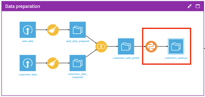
Data preparation

The Data preparation Flow Zone contains two input datasets: web_data and customers_data. These datasets contain customer information, such as customer web usage and revenue.

A data analyst colleague has cleaned these datasets and performed some preliminary preparation on them. In this quick start, a data scientist will perform some feature engineering on these datasets and use them to build a machine learning (ML) model that predicts whether a customer will generate high revenue.

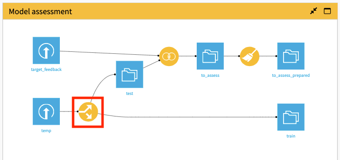
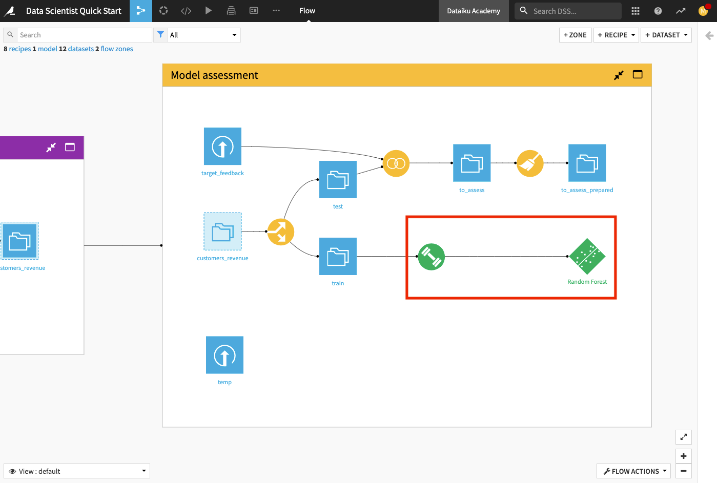
Model assessment

The Model assessment Flow Zone contains two input datasets: target_feedback and temp. The target_feedback dataset contains the ground truth (or true labels) for a test dataset used to evaluate the ML model’s performance. On the other hand, temp is a placeholder and will be replaced by an intermediate dataset in the Flow.

In the Model assessment Flow Zone, the data analyst has created a to_assess_prepared dataset that contains the test data and their true labels. This dataset will be used for evaluating the true test performance of the ML model

Perform Exploratory Data Analysis (EDA) Using Code Notebooks

Sometimes it’s difficult to spot broader patterns in the data without doing a time-consuming deep dive. Dataiku DSS provides the tools for understanding data at a glance using advanced exploratory data analysis (EDA).

This section will cover code notebooks in Dataiku DSS and how they provide the flexibility of performing exploratory and experimental work using programming languages such as SQL, SparkSQL, Python, R, Scala, Hive, and Impala in Dataiku DSS.

Tip

In addition to using a Jupyter notebook, Dataiku DSS offers integrations with other popular Integrated Development Environments (IDEs) such as Visual Studio Code, PyCharm, Sublime Text 3, and RStudio.

Use a Predefined Code Notebook to Perform EDA

• Open the customers_web_joined dataset to explore it.

Notice that the training and testing data are combined in this dataset, with missing revenue values for the “testing” data. We’ll be interested in predicting whether the customers in the “testing” data are high-value or not, based on their revenue.

Let’s perform some statistical analysis on the customers_web_joined dataset by using a predefined Python notebook.

• Return to the Flow.

• In the Data preparation Flow Zone, click the customers_web_joined dataset once to select it, then click the left arrow at the top right corner of the page to open the right panel.

• Click Lab to view available actions.

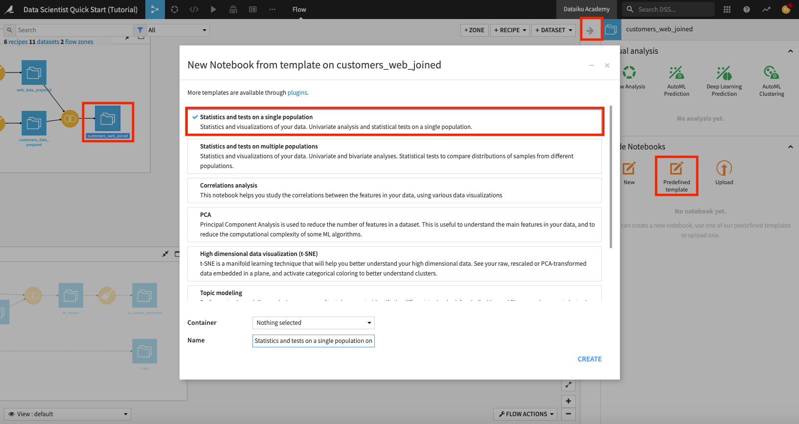
• In the “Code Notebooks” section, select Predefined template.

• In the “New Notebook” window, select Statistics and tests on a single population.

• Rename the notebook to “statistical analysis of customers_web_joined” and click Create.

Dataiku DSS opens up a Jupyter notebook that is prepopulated with code for statistical analysis.

Warning

The predefined Python notebooks in Dataiku DSS are written in Python 2. If your notebook’s kernel uses Python 3, you’ll have to modify the code in the notebook to be compatible with Python 3. Alternatively, if you have a code environment on your instance that uses Python 2, feel free to change the notebook’s kernel to use the Python 2 environment.

Note

Dataiku DSS allows you to create an arbitrary number of Code environments to address managing dependencies and versions when writing code in R and Python. Code environments in Dataiku DSS are similar to the Python virtual environments. In each location where you can run Python or R code (e.g., code recipes, notebooks, and when performing visual machine learning/deep learning) in your project, you can select which code environment to use.

See Setting a Code Environment for details on how to set up Python and R environments and use them in Dataiku DSS objects.

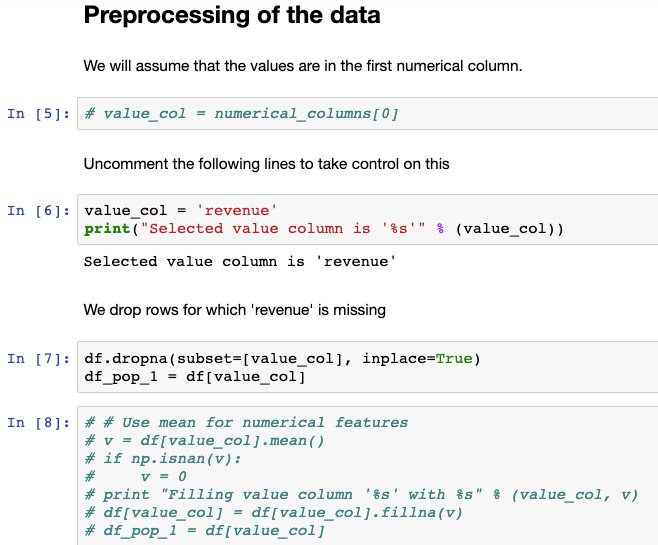
In this notebook, we’ll make the following code modifications:

• Go to the “Preprocessing of the data“ section in the notebook and specify the revenue column to be used for the analysis.

• Instead of imputing missing values for revenue, drop the rows for which revenue is empty (that is, drop the “testing” data rows).

• Enclose all the print statements in the notebook in parenthesis for compatibility with Python 3.

The following figure shows these changes for the “Preprocessing of the data“ section in the notebook.

You can make these code modifications in your code notebook, or you can select the pre-made final_statistical analysis of customers_web_joined notebook to see the final result of performing these modifications. To find the pre-made notebook:

• Click the code icon (</>) in the top navigation bar to open up the “Notebooks” page that lists all the notebooks in your project.

Tip

You can also create notebooks directly from the Notebooks page by using the + New Notebook button.

• Click to open the final_statistical analysis of customers_web_joined notebook.

• Run all the cells to see the notebook’s outputs.

Similarly, you can perform a correlation analysis on the customers_web_joined dataset by selecting the Correlations analysis predefined template from the Lab. You can also see the result of the correlation analysis by viewing the project’s pre-made correlation analysis notebook. To do so,

• Open the final_correlation analysis of customers_web_joined notebook from the notebooks page.

• Run the cells of the pre-made notebook.

Notice that revenue is correlated only with the price_first_item_purchased column. There are also other charts that show scatter matrices etc.

You should also explore the buttons at the top of the notebook to see some of the additional useful notebook features.

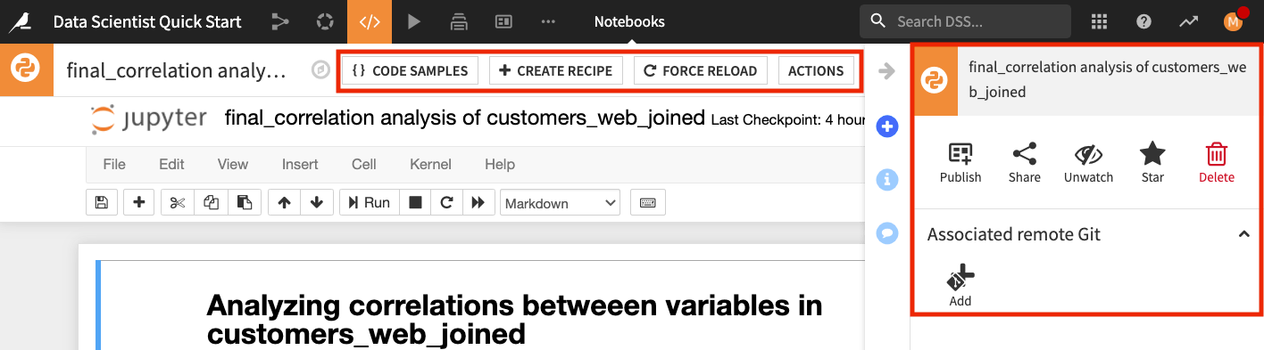
For example, the Code Samples button gives you access to some inbuilt code snippets that you can copy and paste into the notebook, as well as the ability to add your own code snippets; the Create Recipe button allows you to convert a notebook to a code recipe (we’ll demonstrate this in the next section), and the Actions button opens up a panel with shortcuts for you to publish your notebook to dashboards that can be visible to team members, sync your notebook to a remote Git repository, and more.

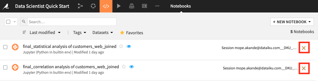
Tip

When you’re done exploring the notebooks used in this section, remember to unload them so that you can free up RAM. You can do this by going to the Notebooks page and clicking the “X” next to a notebook’s name.

Engineer Features Using Code Notebooks and Code Recipes

As a data scientist, you’ll often want to perform feature engineering in addition to the data cleaning and preparation done by a data analyst. Dataiku provides various visual and code recipes that can help to engineer new features quickly.

This section will explore code notebooks further and show how to convert them to code recipes. We’ll also demonstrate how Dataiku DSS helps speed you to value through the use of some important features, namely:

• APIs that allow you to easily interact with objects in your project via code; and

• Project variables that can be reused in Dataiku objects.

Explore a Python Notebook

Here we’ll explore a notebook that creates a target column based on the customers’ revenue. To access the notebook,

• Go to the project’s notebooks by clicking the code icon (</>) in the top navigation bar.

• Open the existing compute_customers_revenue notebook.

Dataiku DSS comes with a complete set of Python APIs.

Note

In parts of DSS where you can write Python code (e.g., recipes, notebooks, scenarios, and webapps) the Python code interacts with DSS (e.g., to read, process, and write datasets) using the Python APIs of DSS.

Dataiku DSS also has APIs that work with R and Javascript. See Dataiku APIs to learn more.

We’ve used a few of these Python APIs in this notebook, some of these include:

• The dataiku package that exposes an API containing modules, functions, and classes that we can use to interact with objects in our project.

• The Dataset class that is used to read the customers_web_joined dataset and create an object.

• The get_dataframe method that is applied to the object and used to create a dataframe.

The Dataiku API is very convenient for reading in datasets regardless of their storage types.

Additionally, this project uses a project variable revenue_value which we’ve defined to specify a revenue cut-off value of 170.

Tip

To see the project variable, go to the More Options (…) menu in the top navigation bar and click Variables.

Note

Variables in Dataiku DSS are containers for information that can be reused in more than one Dataiku DSS object (e.g., recipes, notebooks, and scenarios), making your workflow more efficient and automation tasks more robust. Variables can also be defined, called, and updated through code, such as in code-based recipes.

Lastly, the create_target function in the notebook computes a target column based on the revenue column, so that customers with revenue values that meet or exceed the cut-off value are labeled as high-value customers.

Convert a Notebook to a Code Recipe

One of the powerful features of notebooks is that we can convert them to recipes, thereby applying them to datasets in our Flow and producing outputs. This feature provides value to coders and non-coders alike, as the visual representation of the recipe in the Flow makes it easy for anyone to understand the data pipeline.

We’ll convert the compute_customers_revenue notebook to a Python recipe by applying it to the customers_web_joined dataset. To do this:

• Click the + Create Recipe button at the top of the notebook.

• Click OK to create a Python recipe.

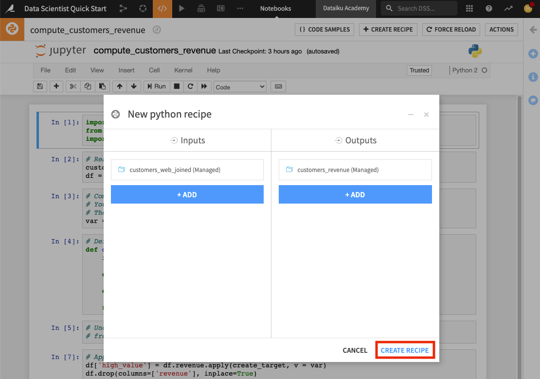
• Click + Add in the “Inputs” column and select customers_web_joined.

• In the “Outputs” column, click + Add to add a new dataset, then name it customers_revenue.

• Specify the CSV format and click Create Dataset.

• Click Create Recipe

The code recipe editor opens up, and here we can see the code from the Python notebook. Notice that in creating the recipe, Dataiku DSS has included some additional lines of code in the editor. These lines of code make use of the Dataiku API to write the output dataset of the recipe.

Modify the code to provide the proper handle for the dataframe.

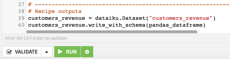
• Scroll to the last line of code.

• Change it to customers_revenue.write_with_schema(df).

• Click Save.

You can also explore the tabs at the top of the Python recipe to see some of its additional features. In particular, the Advanced tab allows you to specify the Python code environment to use, container configuration, and more. We’ll keep the default selections in the “Advanced” tab.

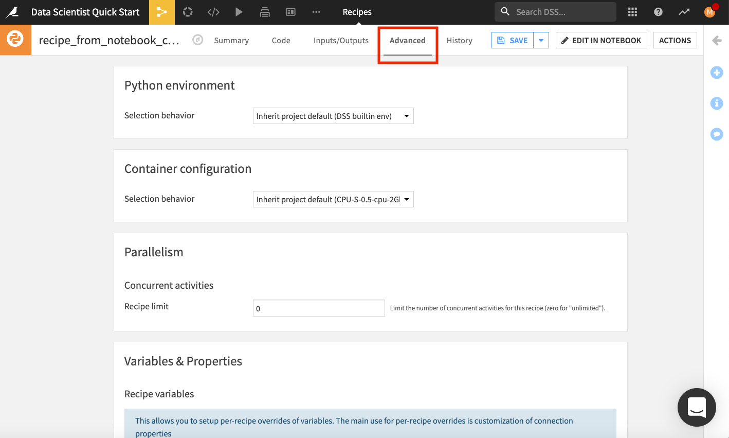
The History tab also tracks changes that are made to the recipe.

Back in the Code tab of the recipe, the left panel lists the input and output datasets. We can also inspect all the variables that are available for use in this recipe. To do so,

• In the left panel, go to the Variables tab.

• Click Validate at the bottom of the editor.

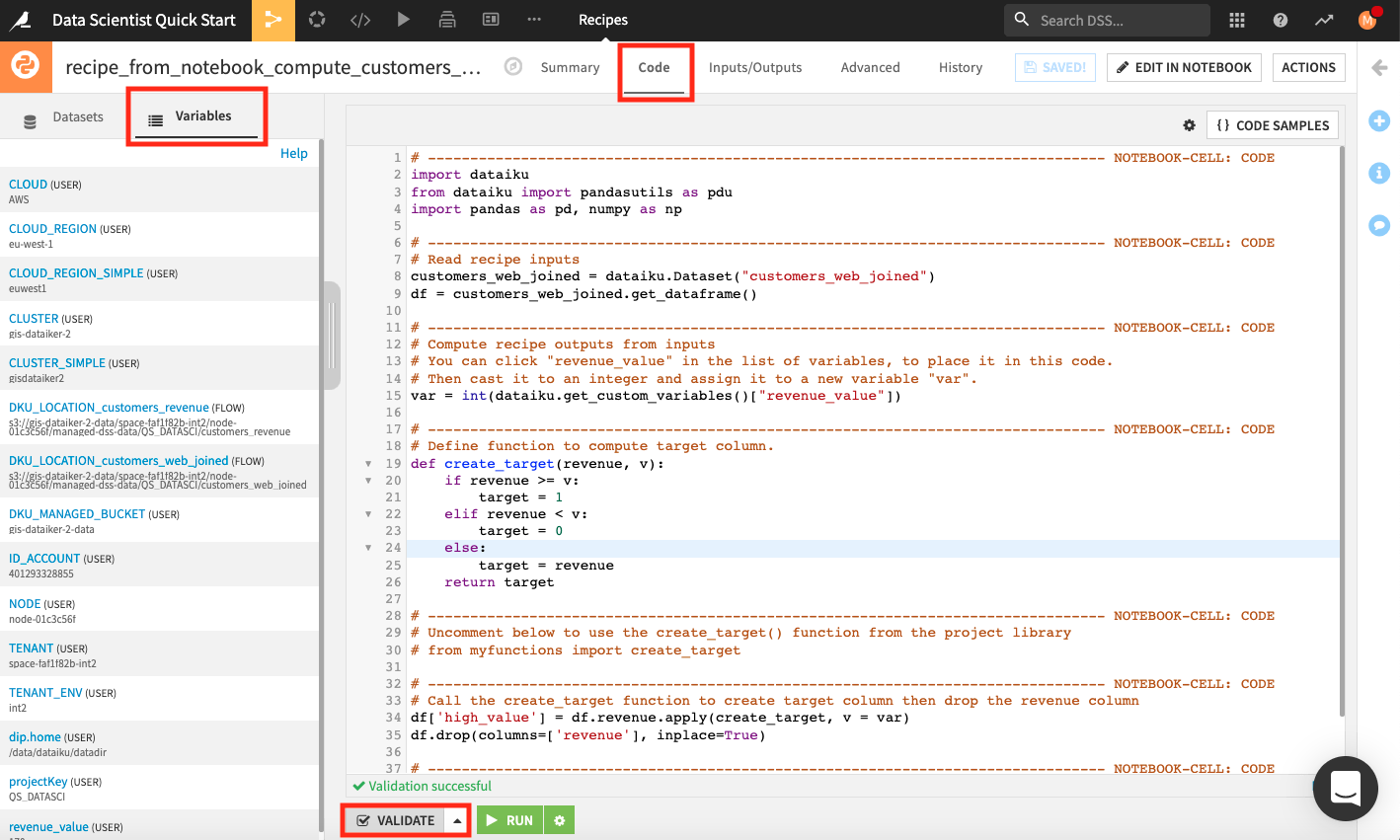
Dataiku DSS validates the script in the code editor and populates the left panel with a list of variables that we can use in the recipe.

• Click Run to run the recipe.

• Wait while the job completes, then open the new dataset called customers_revenue to see the new column high_value.

• Return to the Flow to see that the Python recipe and output are now added to the “Data preparation” Flow Zone.

Tip

When you’re done exploring the notebook used in this section, remember to unload it so that you can free up RAM. You can do this by going to the Notebooks page and clicking the “X” next to a notebook’s name.

Reuse Functions from Code Libraries

As data scientists and coders, you will be familiar with the notion of code libraries for storing code that can be reused in different parts of your project. This feature is available in Dataiku DSS in the form of Project libraries.

This section will explore how coders can create and import existing code libraries for reuse in code-based objects in Dataiku DSS.

Create a Project Library

As we saw in the last section, the Python recipe contains a create_target function that computes a target column by comparing the revenue values to a cut-off value.

Let’s create a similar function in a project library so that the function is available to be reused in code-based objects in Dataiku DSS.

Note

A Project Library is the place to store code that you plan to reuse in code-based objects (e.g., code recipes and notebooks) in your project. You can define objects, functions, etc., in a project library.

Project libraries should be used for code that is project-specific. However, libraries also leverage shared GitHub repositories, allowing you to retrieve your classes and functions.

You can import libraries from other Dataiku DSS projects to use in your project. See the product documentation to learn about reusing Python code and reusing R code.

To access the project library,

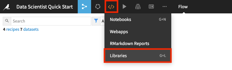
• Go to the “code” icon in the top navigation bar and click Libraries from the dropdown menu.

In the project library,

• Click the dropdown arrow next to the “python” folder to see an existing Python module myfunctions.py containing a function bin_values.

You can create additional Python or R modules in the library. For example, if you’d like to add another Python module:

• Click the +Add button and select Create file.

• Provide a file name that ends in the .py extension and click Create.

• Right-click the new file and select Move.

• Select the folder location for the file and click Move.

• Type your code into the editor window and click Save All.

Note

For code that has been developed outside of Dataiku DSS and is available in a Git repository, see the Cloning a Library from a Remote Git Repository article to learn how to import into a Dataiku Project library.

Use the Module From the Project Library

Now we’ll go back to the existing Python recipe, where we’ll use the bin_values function from the myfunctions_py module.

• Click the Flow icon to return to the Flow.

• Double click the Python recipe to open it.

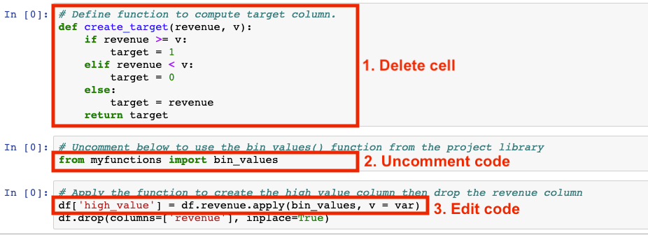
• Click Edit in Notebook and make the following modifications:

  1. Delete the cell where the create_target function is defined.

  2. Uncomment the line from myfunctions import bin_values to import the module and function from your project library.

  3. In the next cell, apply the bin_values function to the revenue column.

• Click Save Back to Recipe.

• Run the recipe.

• After the job completes, you can open the customers_revenue dataset to see that the high_value column contains the values that were previously there.

• Return to the Flow.

Customize the Design of Your Predictive Model

The kinds of predictive modeling to perform in data science projects vary based on many factors. As a result, it is important to be able to customize machine learning models as needed. Dataiku DSS provides this capability to data scientists and coders via coding and visual tools.

In this section, you’ll see one way that Dataiku DSS makes it possible for you to customize aspects of the machine learning workflow using code notebooks.

Split the Training and Testing Data

Before implementing the machine learning part, we first need to split the data in customers_revenue into training and testing datasets. For this, we’ll apply the Split Recipe in Dataiku DSS to customers_revenue.

For convenience, we won’t create the Split recipe from scratch. Instead, we’re going to use the existing Split recipe that is currently applied to the temp dataset in the Model assessment Flow zone. To do this, we’ll change the input of the Split recipe to customers_revenue.

• In the Model assessment Flow Zone, open the Split recipe.

• Switch to the Input/Output tab of the recipe.

• Click Change and select customers_revenue.

• Click Save, accepting the Schema changes, if prompted.

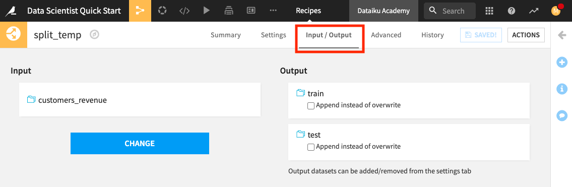
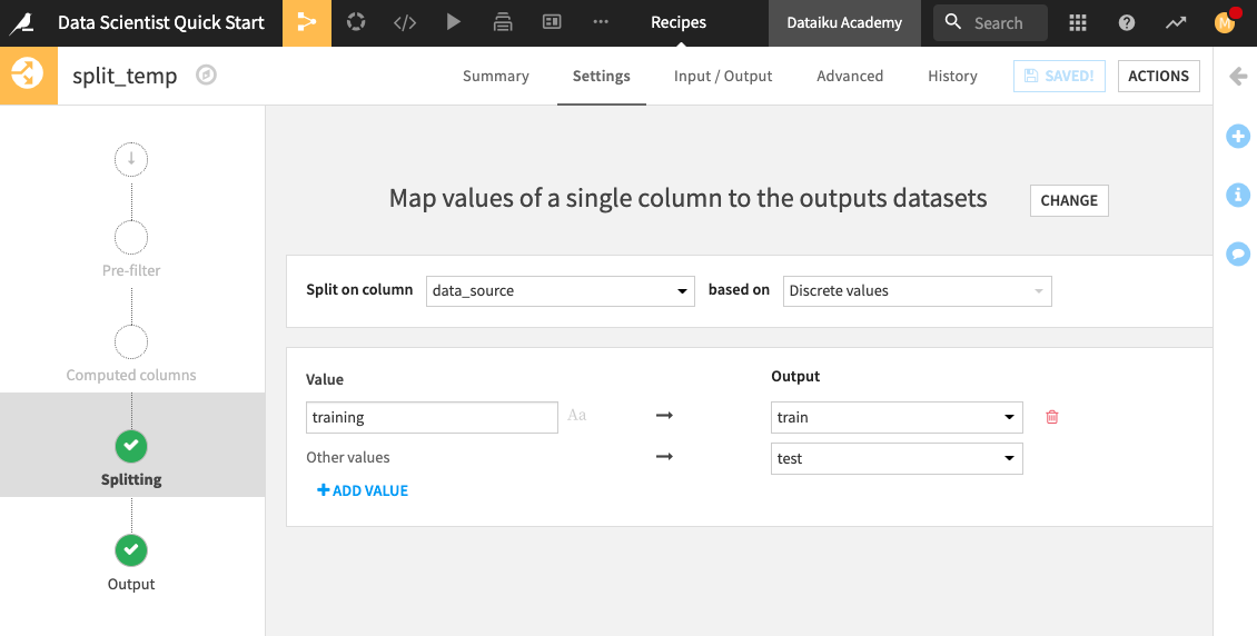
• Click Settings to return to the recipe’s settings.

Notice that the customers_revenue dataset is being split on the data_source column. The customers with the “training” label are assigned to the train dataset, while others are assigned to the test dataset.

• Click Run to update the train and test datasets.

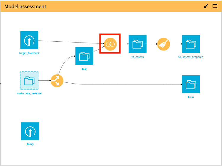
• Return to the Flow.

In the “Model assessment” Flow Zone, notice that the updated train and test datasets are now the outputs of splitting customers_revenue.

Because we updated the train and test datasets, we need to propagate these changes downstream in the “Model assessment” Flow Zone. By doing this, we will update the preliminary data cleaning that the data analyst previously performed.

• In the Model assessment Flow Zone, right-click the Join recipe, then select Build Flow outputs reachable from here.

• Click Build.

Let’s build out our machine learning pipeline. We’ll start by exploring the option of using a Jupyter notebook.

Customize the Design of Your Predictive Model Using a Notebook

As we saw in previous sections, we can create Python notebooks and write code to implement our processing logic. Now, we’ll see how Dataiku DSS allows the flexibility of fully implementing machine learning steps. Let’s explore the project’s custom random forest classification notebook.

• Click the Code icon (</>) in the top navigation bar.

• Click custom random forest classification to open the notebook.

This notebook uses the dataiku API and imports functions from various scikit-learn modules.

A subset of features has been selected to train a model on the train dataset, and some feature preprocessing steps have been performed on this subset.

To train the model, we’ve used a random forest classifier and implemented grid search to find the optimal model parameter values.

To score the model, we’ve used the to_assess_prepared dataset as the test set because it contains the test data and the ground truth prediction values which will be used after scoring to assess the model’s performance.

• Run the cells in the notebook to see the computed AUC metric on the test dataset.

Tip

When you’re done exploring the notebook used in this section, remember to unload it so that you can free up RAM. You can do this by going to the Notebooks page and clicking the “X” next to a notebook’s name.

Note

You can also build your custom machine learning model (preprocessing and training) entirely within a code recipe in your Flow and use another code recipe for scoring the model. For an example that showcases this usage, see the sample project: Build a model using 5 different ML libraries.

Customize the Design of Your Predictive Model Using Visual ML

The process of building and iterating a machine learning model using code can quickly become tedious. Besides, keeping track of the results of each experiment when iterating can quickly become complex. The visual machine learning tool in Dataiku DSS simplifies the process of remembering the feature selection and model parameters alongside performance metrics so that you can easily compare models side-by-side and reproduce model results.

This section will explore how you can leverage this visual machine learning tool to perform custom machine learning. Specifically, we’ll discover how to:

• Train several machine learning models in just a few steps;

• Customize preprocessing and model design using either code or the visual interface;

• Assess model quality using built-in performance metrics;

• Deploy models to the Flow for scoring with test datasets; and so much more.

Train Machine Learning Models in the Visual ML Tool

Here, we’ll show various ways to implement the same custom random forest classifier that we manually coded in the Python notebook (in the previous section). We’ll also implement some other custom models to compare their performance.

• Select the train dataset in the Model assessment Flow Zone.

• Open the right panel and click Lab.

• Select AutoML Prediction from the “Visual analysis” options.

• In the window that pops up, select high_value as the feature on which to create the model.

• Click the box for Interpretable Models for Business Analysts.

• Name the analysis high value prediction and click Create.

Note

When creating a predictive model, Dataiku allows you to create your model using AutoML or Expert mode.

In the AutoML mode, DSS optimizes the model design for you and allows you to choose from a selection of model types. You can later modify the design choices and even write custom Python models to use during training.

In the Expert mode, you’ll have full control over the details of your model by creating the architecture of your deep learning models, choosing the specific algorithms to use, writing your estimator in Python or Scala, and more.

It is worth noting that Dataiku DSS does not come with its own custom algorithms. Instead, DSS integrates well-known machine learning libraries such as Scikit Learn, XGBoost, MLlib, Keras, and Tensor Flow.

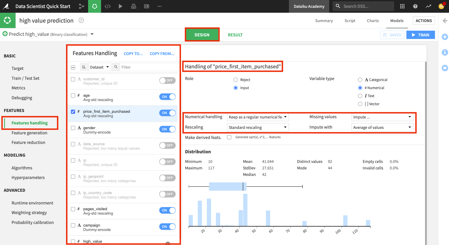
• Click the Design tab to customize the design. Here, you can go through the panels on the left side of the page to view their details.

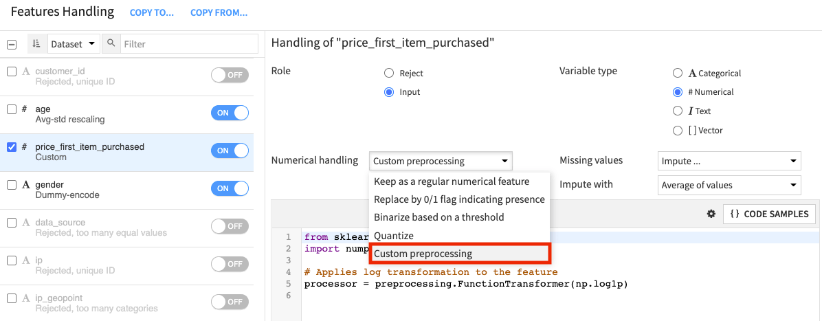
• Click the Features handling panel to view the preprocessing.

Notice that Dataiku has rejected a subset of these features that won’t be useful for modeling. For the enabled features, Dataiku already implemented some preprocessing:

• For the numerical features: Imputing the missing values with the mean and performing standard rescaling

• For the categorical features: Dummy-encoding

If you prefer, you can customize your preprocessing by selecting Custom preprocessing as the type of “Numerical handling” (for a numerical feature) or “Category handling” (for a categorical feature). This will open up a code editor for you to write code for preprocessing the feature.

• Click the Algorithms panel to switch to modeling.

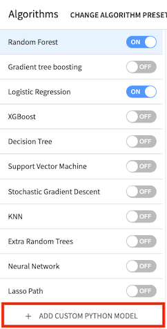
• Enable Random Forest and disable Decision Tree.

We’ll also create some custom models with code in this ML tool.

• Click + Add Custom Python Model from the bottom of the models list.

Dataiku DSS displays a code sample to get you started.

Note

The Code Samples button in the editor provides a list of models that can be imported from scikit-learn. You can also write your model using Python code or import a custom ML algorithm that was defined in the project library. Note that the code must follow some constraints depending on the backend you have chosen (in-memory or MLlib).

Here, we are using the Python in-memory backend. Therefore, the custom code must implement a classifier that has the same methods as a classifier in scikit-learn; that is, it must provide the methods fit(), predict(), and predict_proba() when they make sense.

The Academy course on Custom Models in Visual ML covers how to add and optimize custom Python models in greater detail.

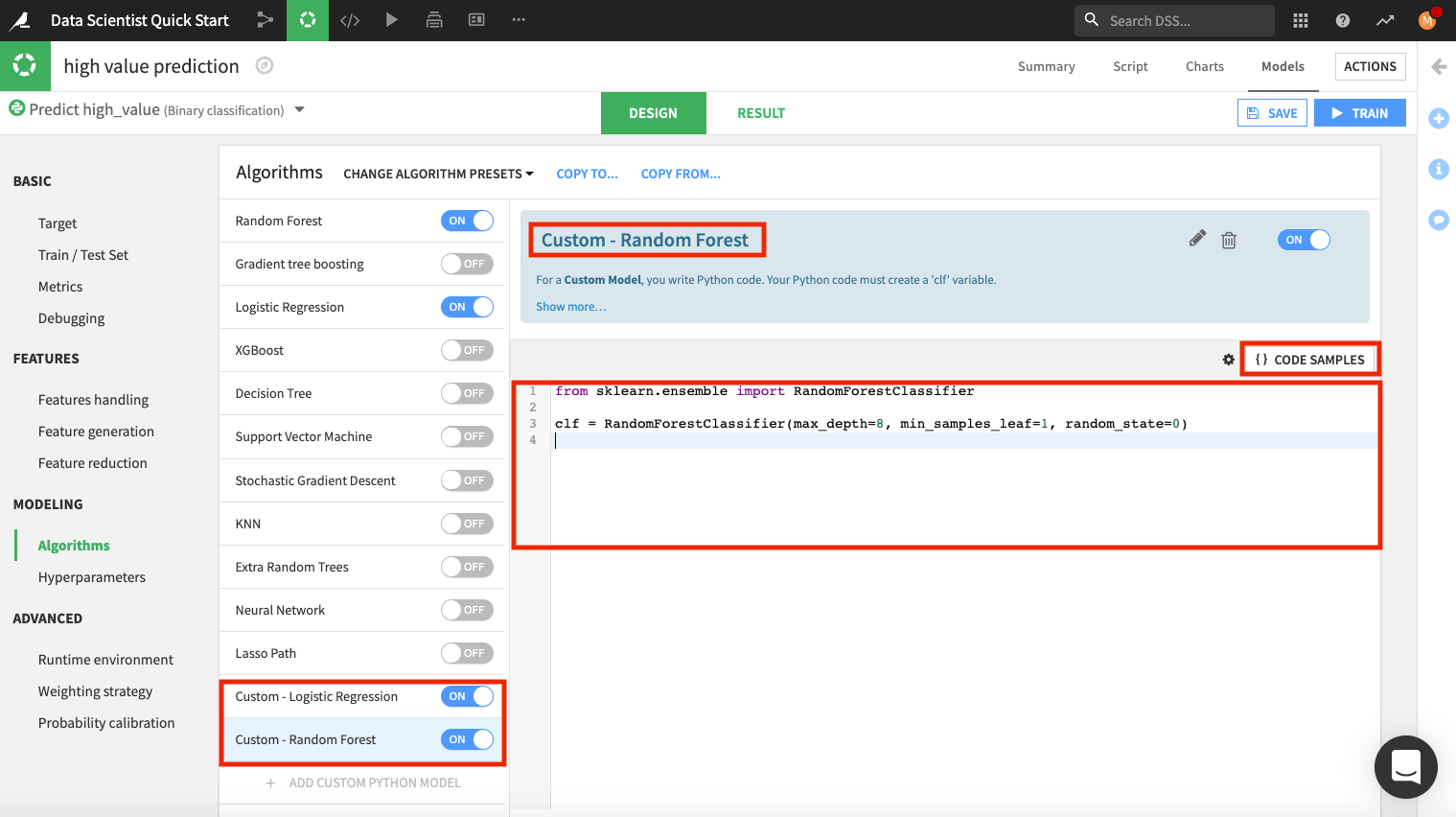
• Click the pencil icon to rename “Custom Python model” to Custom - Logistic Regression.

• Delete the code in the editor and click Code Samples.

• Select Logistic regression and click + Insert.

• Add another custom model. This time, rename the model to Custom - Random Forest.

• Delete the code in the editor and type:

from sklearn.ensemble import RandomForestClassifier
clf = RandomForestClassifier(max_depth=8, min_samples_leaf=1, random_state=0)

• Before leaving this page, explore other panels, such as Hyperparameters, where you can see the “Grid search” strategy being used.

• Also, click the Runtime environment panel to see or change the code environment that is being used.

Tip

The selected code environment must include the packages that you are importing into the Visual ML tool. In our example, we’ve imported libraries from scikit-learn, which is already included in the DSS builtin code environment that is in use.

• Save the changes, then click Train.

• Name the session Customized models and click Train again.

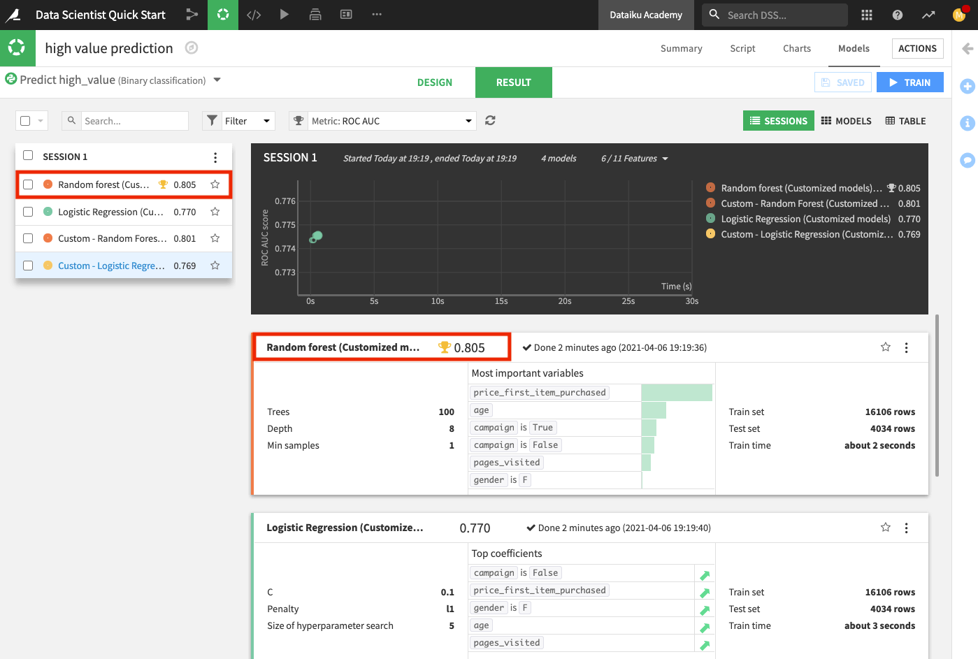
The Result page for the sessions opens up. Here, you can monitor the optimization results of the models for which optimization results are available.

After training the models, the Result page shows the AUC metric for each trained model in this training session, thereby, allowing you to compare performance side by side.

Tip

Every time you train models, the training sessions are saved and listed on the Result page so that you can access the design details and results of the models in each session.

The chart also shows the optimization result for the Logistic Regression model.

Deploy the ML Model to the Flow

Next, we’ll deploy the model with the highest AUC score (the Random forest model) to the Flow to apply it to the test data and evaluate the test data predictions in light of the ground truth classes.

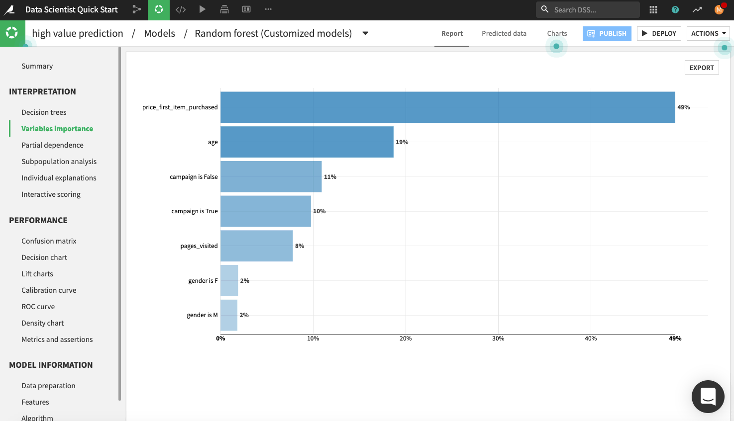
• Click Random forest (Customized model) from the list to go to the model’s Report page.

• Explore the model report’s content by clicking any of the items listed in the left panel of the report page, such as any of the model’s interpretations, performance metrics, and model information.

The following figure displays the “Variables importance” plot, which shows the relative importance of the variables used in training the model. Model interpretation features like those found in the visual ML tool can help explain how predictions are made and ensure that fairness requirements around features (such as age and gender) have been met.

Note

You can automatically generate the trained model’s documentation by clicking the Actions button in the top right-hand corner of the page. Here, you can select the option to Export model documentation. This feature can help you easily document the model’s design choices and results for better information sharing with the rest of your team.

Let’s say, overall, we are satisfied with the model. The next thing to do is deploy the model from the Lab to the Flow.

• Click Deploy from the top right corner of the page, and name the model Random Forest.

• Click Create.

Back in the Flow, you can see that two new objects have been added to the Flow. The green diamond represents the Random Forest model.

Score the ML Model

Now that the model has been deployed to the Flow, we’ll use it to predict new, unseen test data. Performing this prediction is known as Scoring.

• Click the Random Forest model in the Model assessment Flow Zone.

• In the right panel, click Score.

• In the scoring window, specify test as the input dataset.

• Name the output dataset scored and store it in the CSV format.

• Click Create Recipe. This opens up the Settings page.

• Click Run.

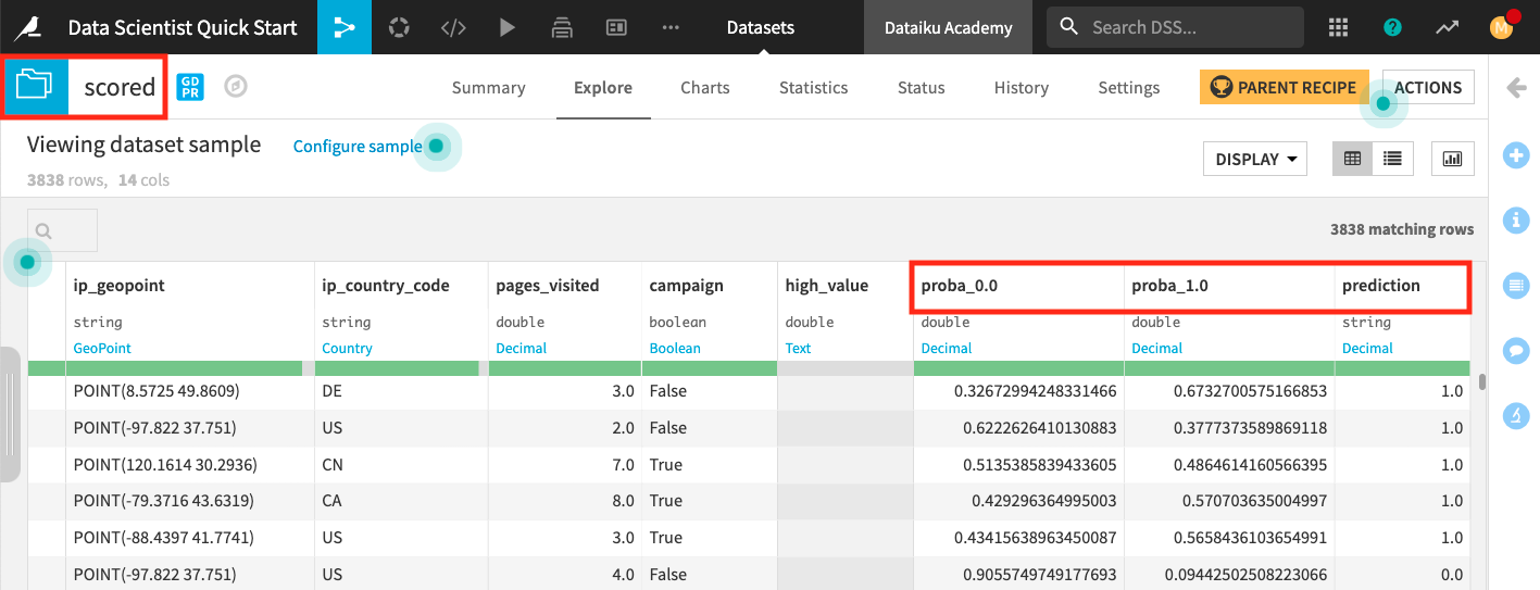
• Wait for the job to finish running, then click Explore dataset scored.

The last three columns of the scored dataset contain the probabilities of prediction and the predicted class.

When you return to the Flow, you’ll see additional icons that represent the Score recipe and the scored dataset.

Evaluate the Model Predictions

For this part, let’s take a look into the Model assessment Flow Zone.

Let’s say that a data analyst colleague created the Flow in this zone so that the to_assess_prepared dataset includes the data for customers in the test dataset and their known classes. We can now use the to_assess_prepared dataset to evaluate the true performance of the deployed model.

We’ll perform the model evaluation as follows.

• Double click the Model assessment Flow Zone to open it.

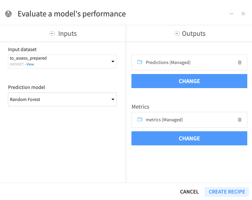
• Click the to_assess_prepared dataset and open the right panel to select the Evaluate Recipe from the “Other recipes” section.

• Select Random Forest as the “Prediction model”.

• Click Set in the “Outputs” column to create the first output dataset of the recipe.

• Name the dataset Predictions and store in CSV format.

• Click Create Dataset.

• Click Set to create the metrics dataset in a similar manner.

• Click Create Recipe.

• When the recipe window opens, click Run.

• Return to the Flow to see that the recipe has output two datasets: the metrics dataset, which contains the performance metrics of the model, and the predictions datasets, which contains columns about the predictions.

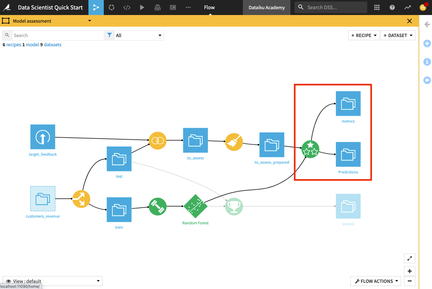
• Open up the metrics dataset to see a row of computed metrics that include the AUC score.

• Return to the Flow and open the Predictions dataset to see the last four columns which contain the model’s prediction of the test dataset.

• Return to the Flow.

Tip

Each time you run the Evaluate recipe, DSS appends a new row of metrics to the metrics dataset.

Automate Active Version of Deployed Model

In this section, we’ll examine Dataiku’s automation features by using a custom scenario. As a data scientist, you’ll find scenarios in Dataiku DSS useful for automating tasks that include: training and retraining models, updating active versions of models in the Flow, building datasets, and so on.

Automate ML Tasks by Using a Scenario

The Project comes with an existing scenario called Automate. To access scenarios in your project,

• From the Flow, go to the Jobs icon in the top navigation bar and click Scenarios. This opens the Scenarios page where you can see existing scenarios and create new ones.

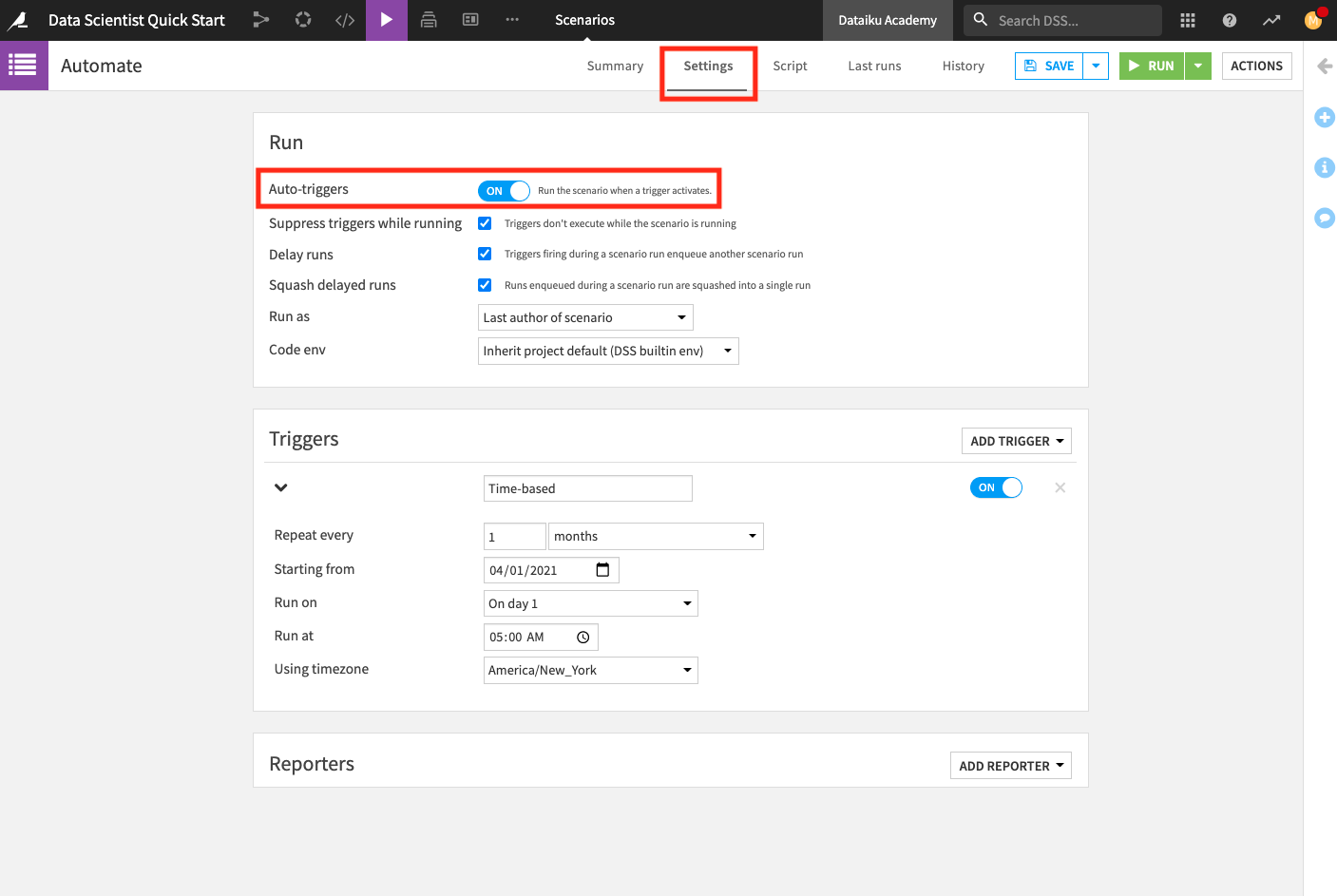
• Click Automate to open the scenario. This opens the scenario’s Settings page. The Settings page is where you define triggers and reporters.

• Optionally, you can enable the “Auto-triggers” so that the scenario automatically runs when the trigger activates. Note that this setting may be disabled in the Dataiku Online edition.

• Click Save.

Note

A scenario has two required components:

• Triggers that activate a scenario and cause it to run, and

• steps, or actions, that a scenario takes when it runs.

There are many predefined triggers and steps, making the process of automating Flow updates flexible and easy to do. For greater customization, you can create your own triggers and steps using Python or SQL.

Reporters are optional components of a scenario. They are useful for setting up a reporting mechanism that notify of scenario results (for example: by sending an email if the scenario fails).

The Automate scenario already has a monthly trigger set up so that the scenario runs every first day of the month.

Dataiku DSS allows you to create step-based or custom Python scenarios. The Automate scenario is Python-based. Let’s explore the script.

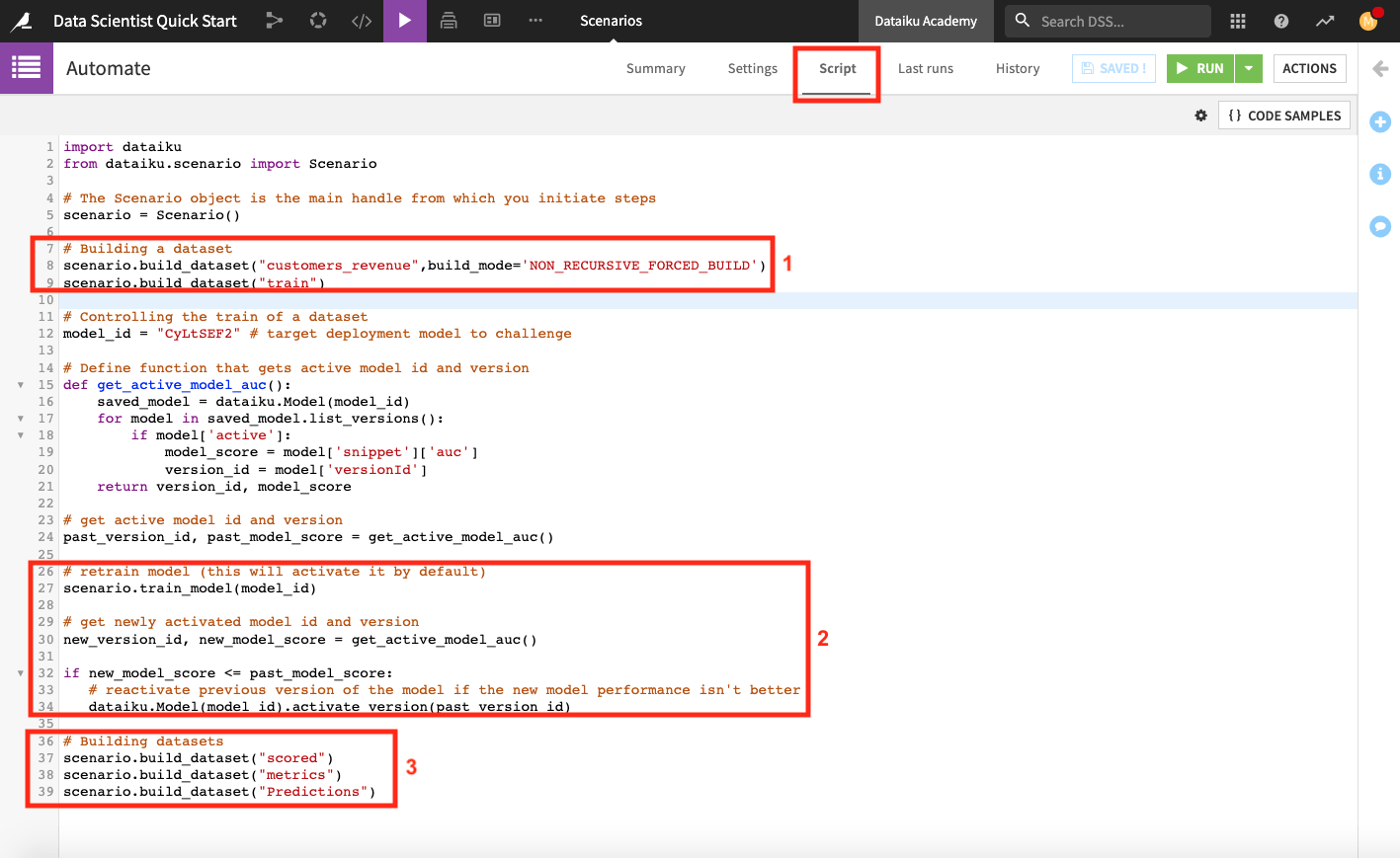
• Click Script at the top of the page to see the scenario’s script.

The scenario script is a full-fledged Python program that executes scenario steps. This script uses the Dataiku API to access objects in the project. The script also uses the scenarios API within the scenario in order to run steps such as building a dataset and training a model.

Note

The scenario API is exclusive to Scenarios, and cannot be used on a Python notebook.

When we run the scenario, it will perform the following tasks.

1. Build the customers_revenue and train dataset. To build the train dataset, the scenario runs its parent recipe (the Split recipe) and therefore builds the test dataset also.

2. Retrain the deployed model and set this new model version as the active version in the Flow only if the new version has a higher AUC score than the previous model version. This step overwrites the default behavior of Dataiku DSS.

Tip

If you go to the “Settings” tab of a model’s page, you can see that by default, Dataiku DSS activates new model versions automatically at each retrain (that is, the most recent model version is set as the active version). However, you have the option of changing this behavior to activate new model versions manually.

3. Build the scored, metrics, and Predictions datasets

Before we run the scenario, we’ll make two changes to the project:

• Replace the model ID on line 12 with that of the deployed model and click Save.

Tip

To find the model ID for your deployed model, return to the Flow and open the model. The URL is of the format: INSTANCE_URL/projects/projectKey/savedmodels/modelID/versions/. You can copy the model ID number from here.

• Change the value of the project variable “revenue_value” from 170 to 100. Because the customers_revenue dataset depends on the value of “revenue_value”, changing the value of “revenue_value” will change the data in customers_revenue.

Recall that you can access the project variable by going to the More actions … menu in the top navigation bar.

The scenario is now ready to use. To test it,

• Return to the Automate scenario from the Jobs menu.

• Click Run and wait for the scenario to complete its jobs.

Tip

You can switch to the Last runs tab of the scenario to follow its progress. Here, you can examine details of the run, what jobs are triggered by each step in the scenario, and the outputs produced at each scenario step.

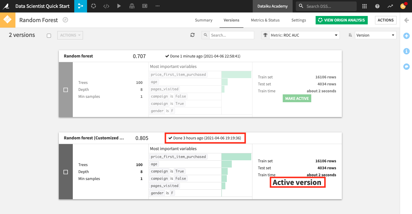
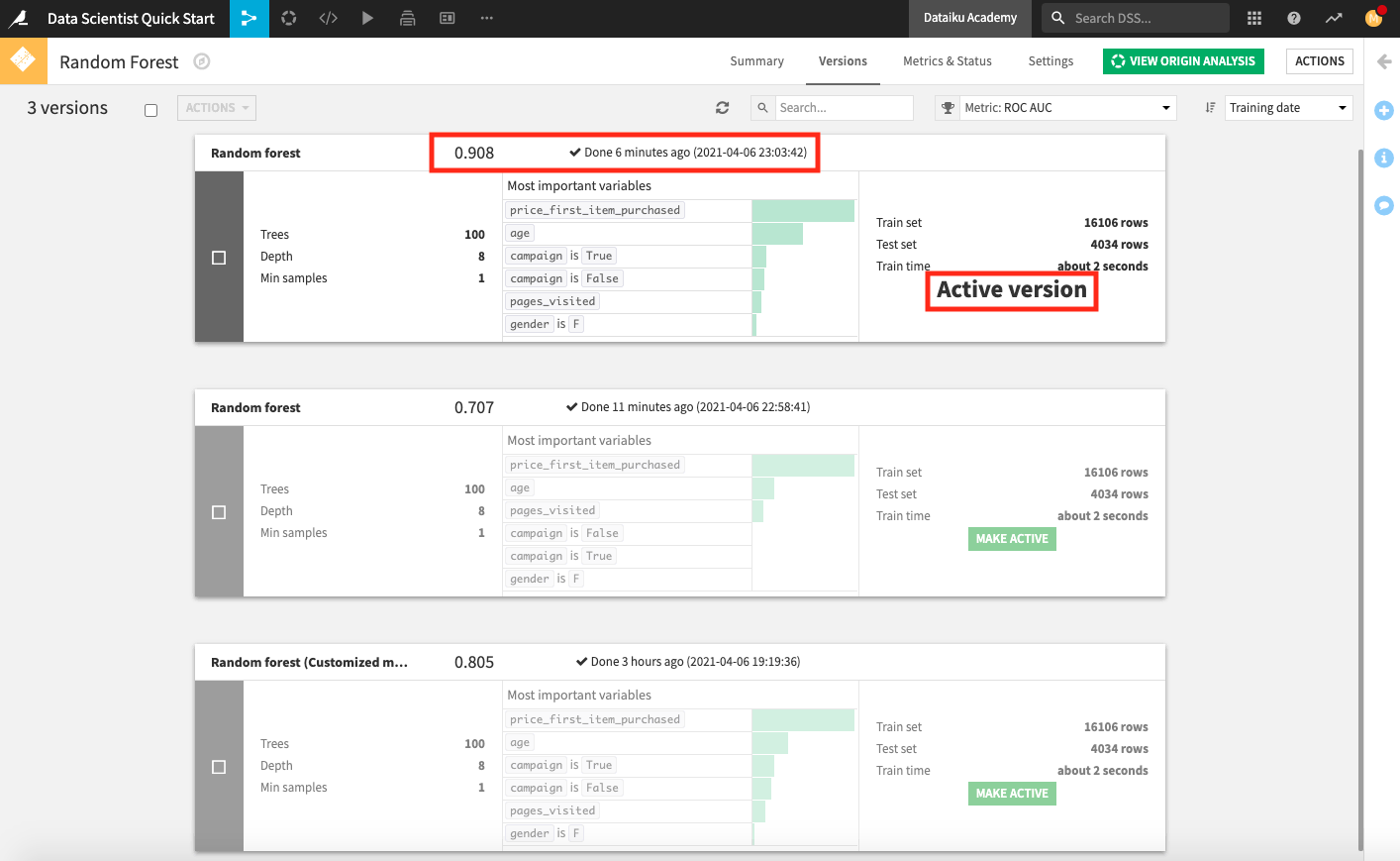
Upon returning to the Flow and opening the deployed model, notice that the older model version remains active as long as its ROC AUC score is not worse than the new version’s ROC AUC score (a consequence of the Python step in the scenario).

• Change the value of the project variable “revenue_value” from 100 to 220.

• Return to the Automate scenario from the Jobs menu.

• Click Run and wait for the scenario to complete its jobs.

• Open the deployed model to see that the new model version, with a higher AUC score than the previous active version, is now active.

• Open the metrics dataset to observe that an additional row of test metrics was added for the active model version each time the scenario ran.

Tip

Over time, we can track scenarios to view patterns of successes and failures. To do so, go to the Jobs menu in the top navigation bar and select Automation Monitoring.

Create Reusable Data Products

This section briefly covers some extended capabilities Dataiku DSS provides to coders and data scientists.

Dataiku’s code integration allows you to develop a broad range of custom components and to create reusable data products such as Dataiku applications, webapps, and plugins.

Dataiku Applications

Dataiku Applications are a kind of DSS customization that allows projects to be reused by colleagues who simply want to apply the existing project’s workflow to new data without understanding the project’s details.

Therefore, a data scientist can convert the project into a Dataiku application so that anyone who wants to use the application only has to create their own instance of the Dataiku application. These applications can take one of two forms:

• Visual Applications that allow you to package a project with a GUI on top

• Applications-as-Recipes that allow you to package part of a Flow into a recipe usable in the Flows of other projects.

Webapps

You can extend the visualization capabilities of Dataiku DSS with interactive webapps. Dataiku DSS allows you to write many kinds of webapps including:

• Standard webapps made at least of HTML, CSS, and Javascript code that you can write in the DSS webapp editor. DSS takes care of hosting your webapp and making it available to users with access to your data project.

• Shiny webapps that use the Shiny R library.

• Bokeh webapps that use the Bokeh Python library.

• Dash webapps that use the Dash Python framework.

The Visualization course covers how to create interactive webapps in Dataiku in detail.

Plugins

Plugins allow you to implement custom components that can be shared with others. Plugins can include components such as dataset connectors, notebook templates, recipes, processors, webapps, machine learning algorithms, and so on.

To develop a plugin, you program the backend using a language like Python or R. Then, you create the user interface by configuring parameters in .json files.

Plugins can be installed from the Dataiku Plugin store (in your Dataiku DSS instance) by uploading a Zip file or downloading from a Git repository.

What’s Next?

Congratulations! In a short amount of time, you learned how Dataiku enables data scientists and coders through the use of:

• Python notebooks for EDA, creating code recipes, and building custom models;

• code libraries for code-reuse in code-based objects;

• the visual ML tool for customizing and training ML models; and

• scenarios for workflow automation.

You also learned about code environments and how to create reusable data products. To review your work, compare your project with the completed project in the Dataiku Gallery.

Your project also does not have to stop here. Some ways to build upon this project are by:

• Documenting your workflow and results in a wiki;

• Creating webapps and Dataiku applications to make assets reusable;

• Sharing output datasets with other Dataiku DSS projects or using plugins to export them to tools like Tableau, Power BI, or Qlik.

Finally, this quick start is only the starting point for the capabilities of Dataiku DSS. To learn more, please visit the Dataiku Academy, where you can find more courses, learning paths and can complete certificate examinations to test your knowledge.