Hands-On: Create the Model
In this lesson, we will create a machine learning model to predict whether or not a new customer will become a high-revenue customer. To do this, we’ll train a classification model using historical customer records and order logs from Haiku T-Shirts. This historical data is known as labeled data. Later, we’ll score the model using unlabeled data.
When evaluating machine learning models, it is helpful to have a baseline model to compare with in order to establish that our models are performing better as we iterate on them.
We do not expect our initial, or baseline, model to be a high-performing model. Throughout the hands-on lessons in this course, we will evaluate and improve the model, implementing checks to ensure its predictions align with business expectations.
After we’ve deployed our best model to the Flow, we’ll score the unlabeled dataset–labeling the customers as True (high revenue) or False (not high revenue). We’ll do this in the scoring section of the ML Practitioner course series.
Business Objectives
It costs more to add new customers than it does to keep existing customers. Therefore, the business wants to target high-revenue Haiku T-shirts customers for the next marketing campaign.
Since the business is focused on finding and labeling (predicting) high-revenue customers, we’ll want to maximize the number of correct predictions while also minimizing the number of times the model incorrectly predicts that a customer is not a high-revenue customer. To do this, we’ll pay close attention to the confusion matrix when evaluating model results.
The business also wants to be able to measure how well the model is aligning with business expectations for specific known cases.
To enable this measurement, we’ll take advantage of Dataiku DSS’ built-in model diagnostics such as model assertions. Model assertions, or ML assertions, act as a “sanity check” to ensure predictions align with business expectations for specific known cases.
Machine Learning Objectives
Build a high-performing, interpretable model to predict high-revenue customers.
Minimize false negatives–that is, minimize the number of times the model incorrectly predicts that a customer is not a high revenue customer.
Configure ML assertions.
Prerequisites
This lesson assumes that you have completed Basics 101, 102, and 103, which are part of the Core Designer Learning Path in Dataiku Academy, prior to beginning this one!
Create Your Project
From the Dataiku homepage, click +New Project > DSS Tutorials > ML Practitioner > Machine Learning Basics (Tutorial).
Note
You can also download the starter project from this website and import it as a zip file.
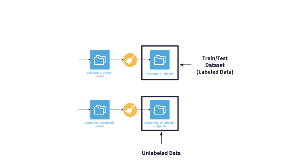
Click on Go to Flow. In the Flow, you can see the steps used in the previous tutorials to create, prepare, and join the customers and orders datasets.
In addition, there is a dataset of “unlabeled” customers representing the new customers that we want to predict. These customers have been joined with the orders log and prepared in much the same way as the historical customer data.
Alternatively, you can continue in the same project you worked on in Basics 103, by
Removing the total_sum and count columns from the customers_labeled dataset.
Downloading a copy of the customers_unlabeled.csv file and uploading it to the project.
Preparing the customers_unlabeled dataset to match the schema of the customers_labeled dataset. Remember to use an inner join to join customers_unlabeled with orders_by_customer. You can even copy-paste the Prepare recipe steps from the script you used to prepare the customers_orders_joined dataset.
Train the Baseline Model
Our goal is to predict (i.e., perform a calculated guess) whether the customer will become a “high revenue” customer. If we can predict this correctly, we would be able to assess the quality of the cohorts of new customers, and help the business more effectively drive acquisition campaigns and channels.
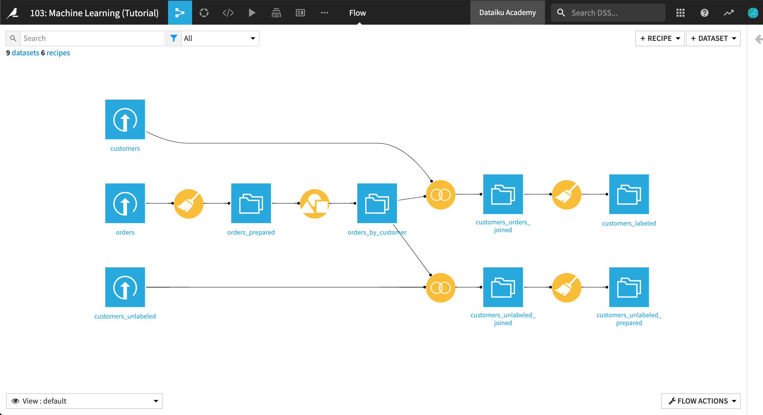
In the Flow, select the customers_labeled dataset and click on the Lab button.
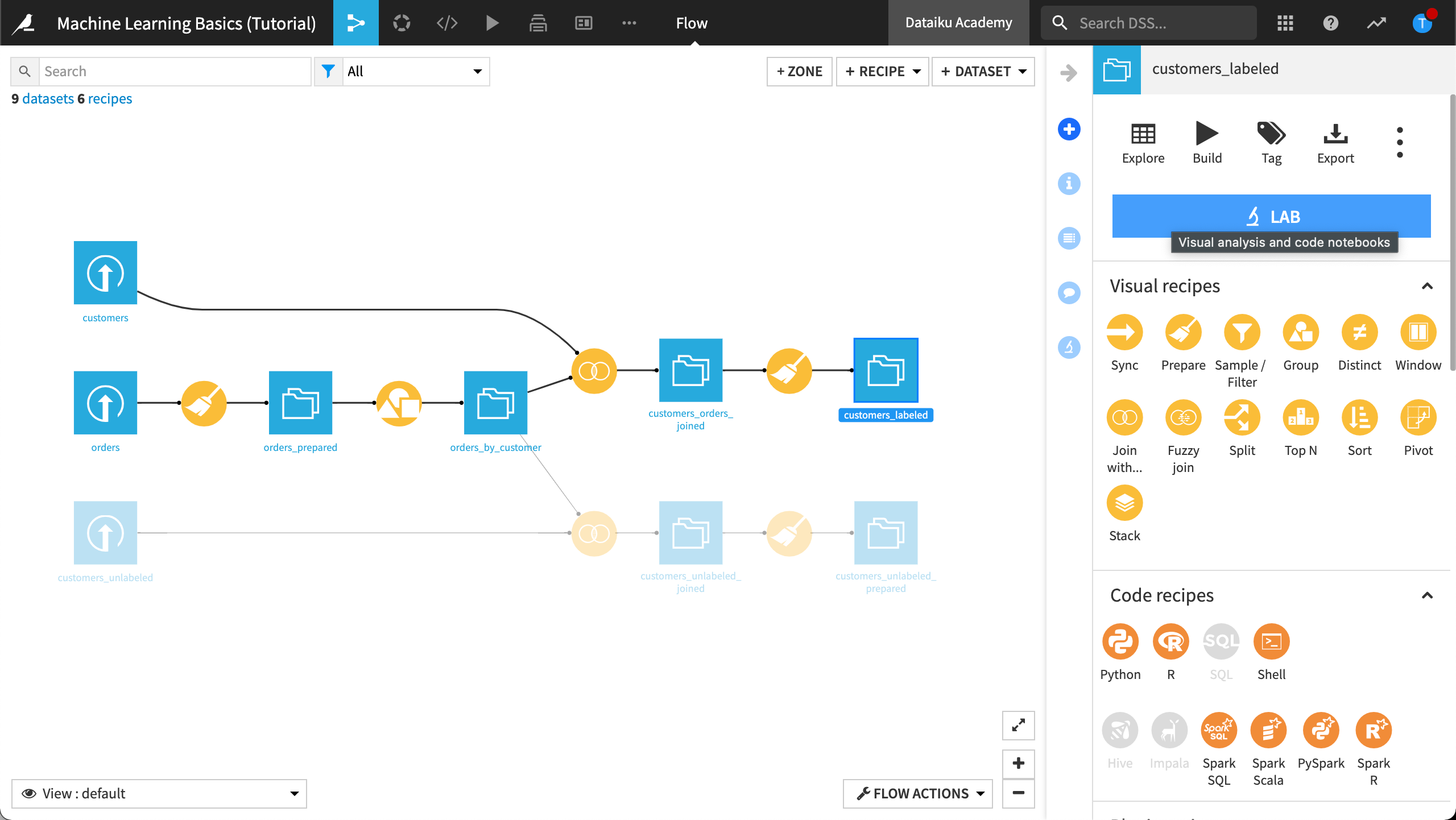
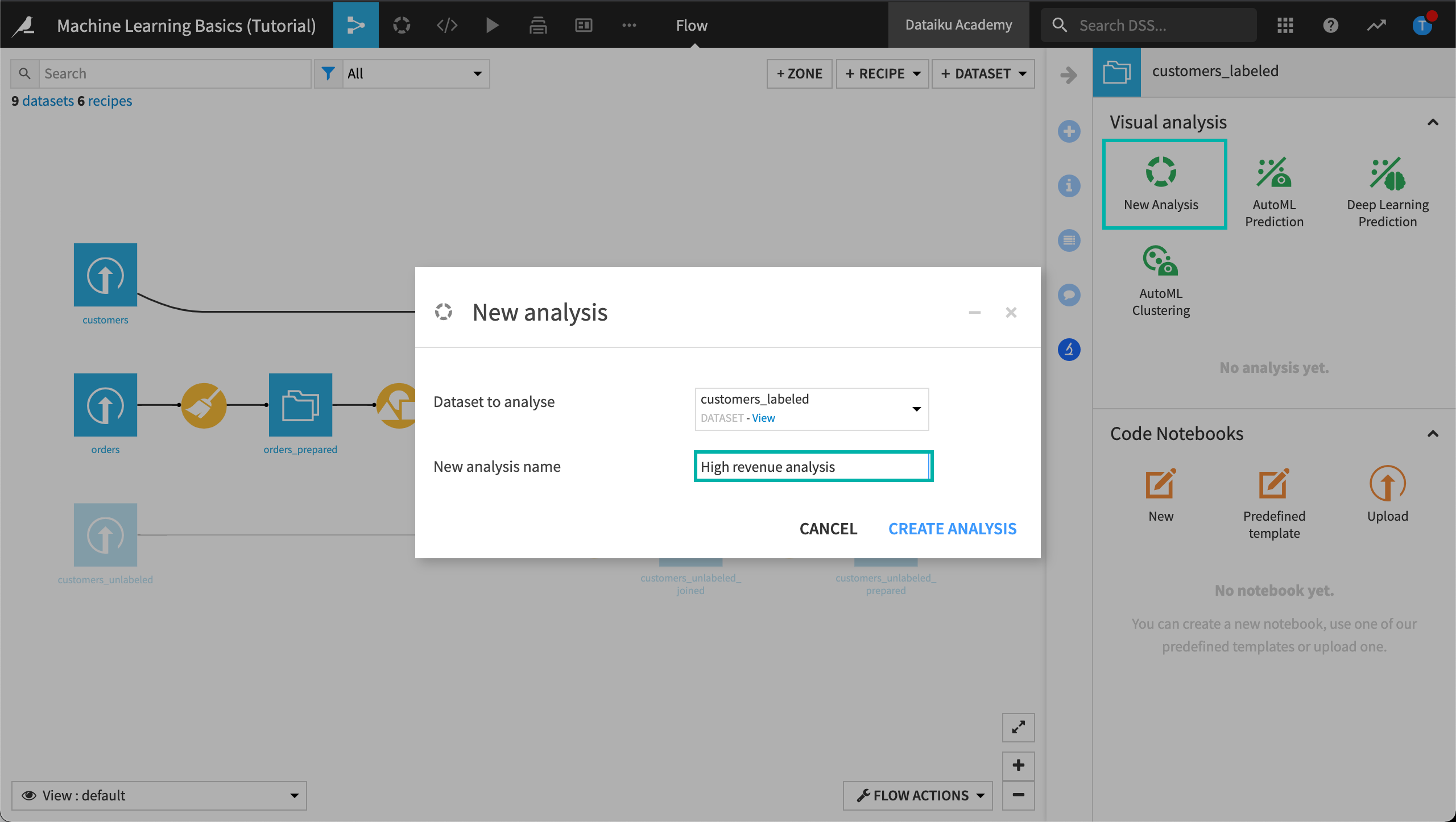
Click New Analysis.
Give the analysis the more descriptive name
High revenue analysis, then click Create Analysis.
Our labeled dataset contains personal information about the customer including the age of their first order, the number of pages visited on average, and whether or not the customer responded to a campaign. The last column high_revenue is a flag for customers generating a lot of revenue based on their purchase history. It will be used as the target variable of our modeling task.
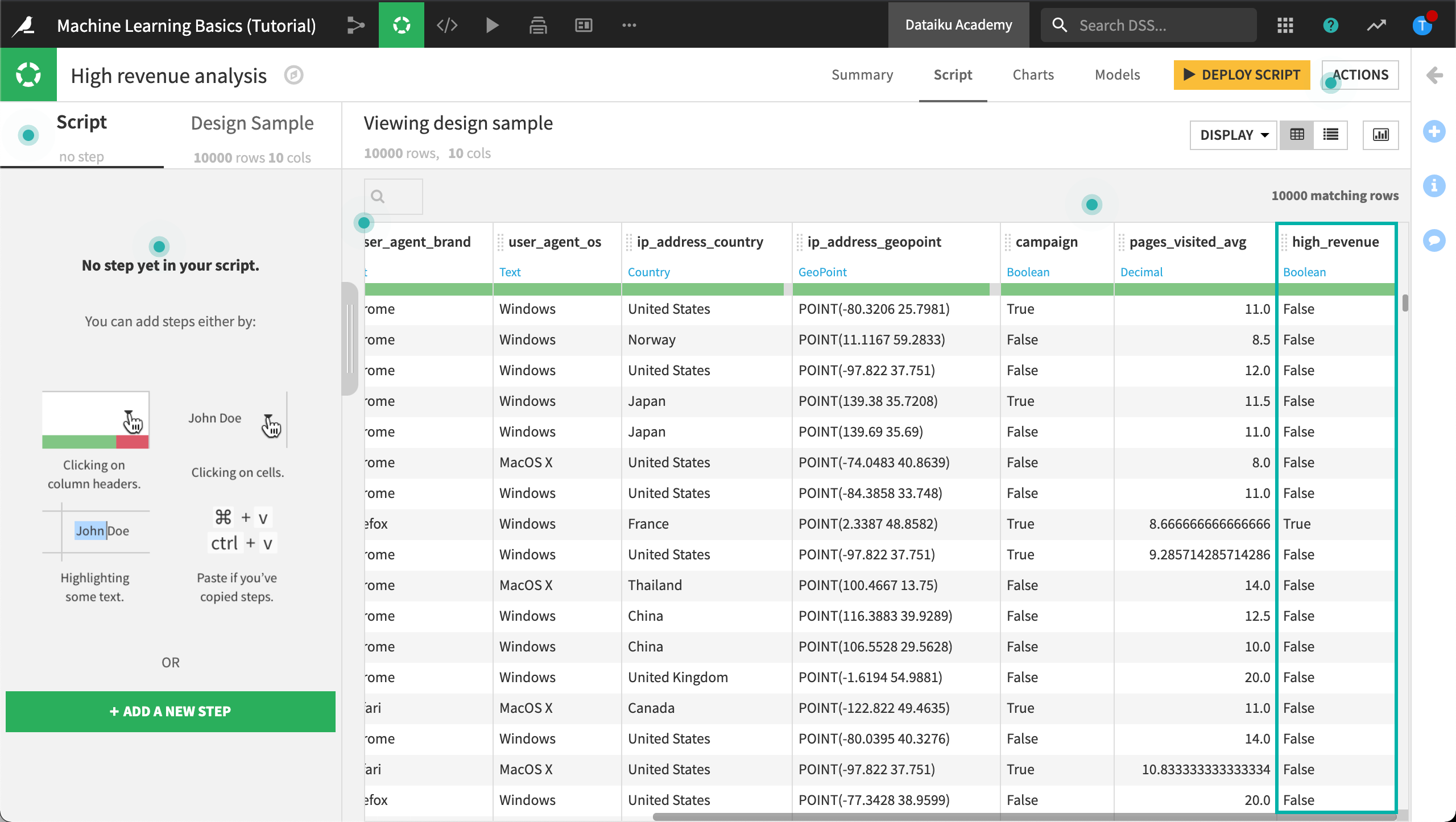
Now let’s build our baseline model!
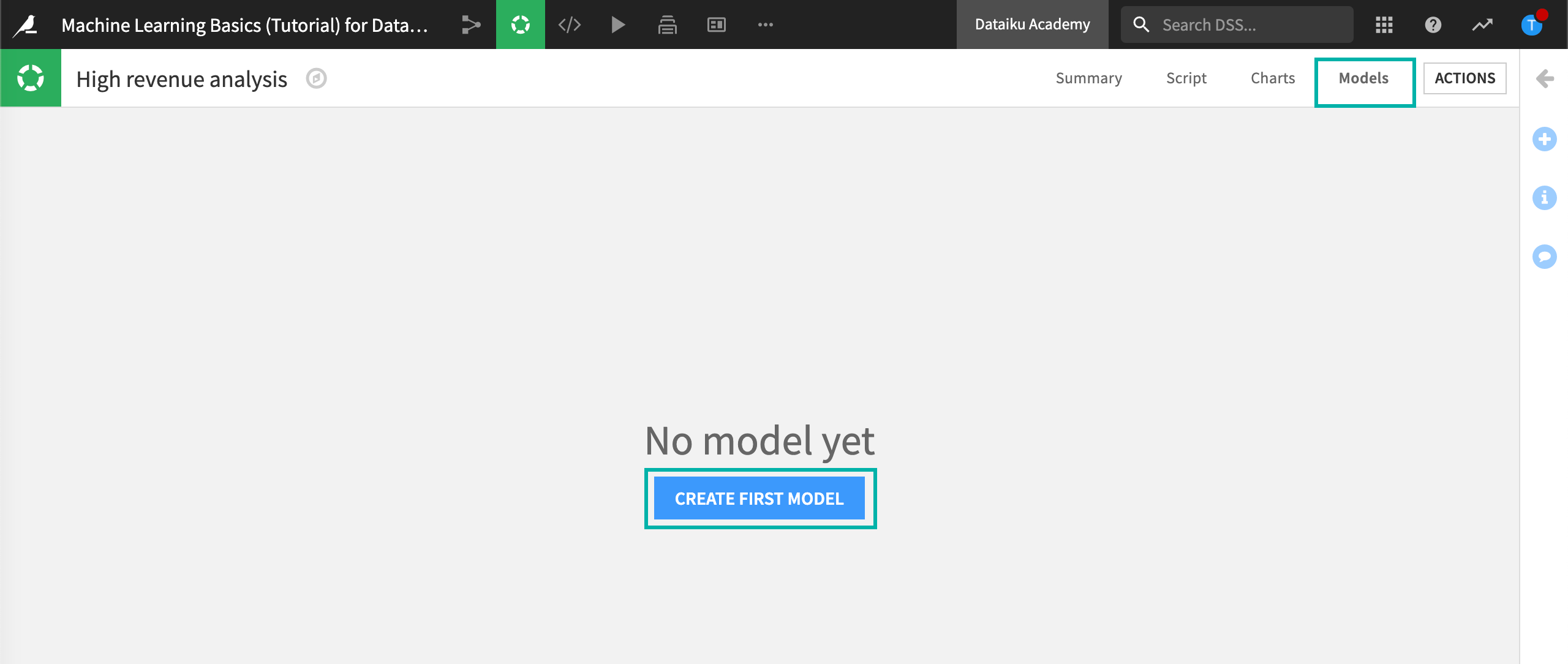
In the top right corner, go to the Models tab and then click Create first model.
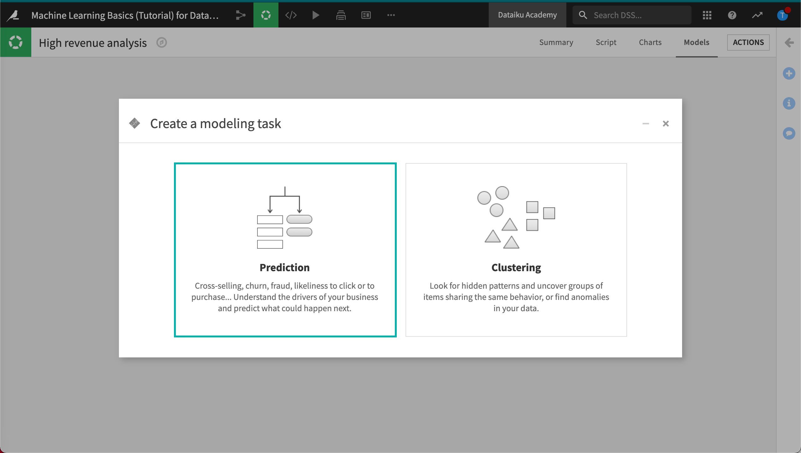
DSS displays Create a modeling task, where you can choose the type of modeling task you want to perform.
Click Prediction since we want to predict high_revenue.
Select high_revenue as the target variable.
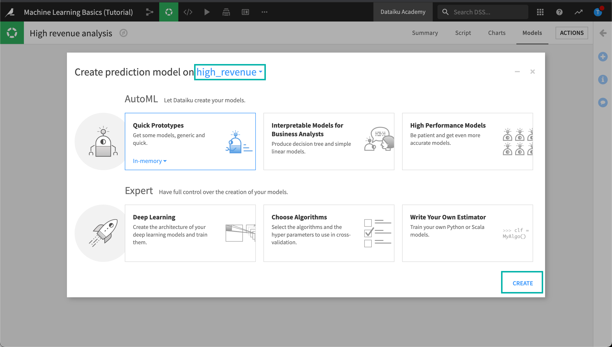
Automated machine learning provides templates to create models depending on what you want to achieve; for example, either using machine learning to get some insights on your data or creating a highly performant model.
Keep the default Quick Prototypes template on the In-memory (Python) backend and click Create.
Click Train on the next screen.
DSS guesses the best preprocessing to apply to the features of your dataset before applying the machine learning algorithms.
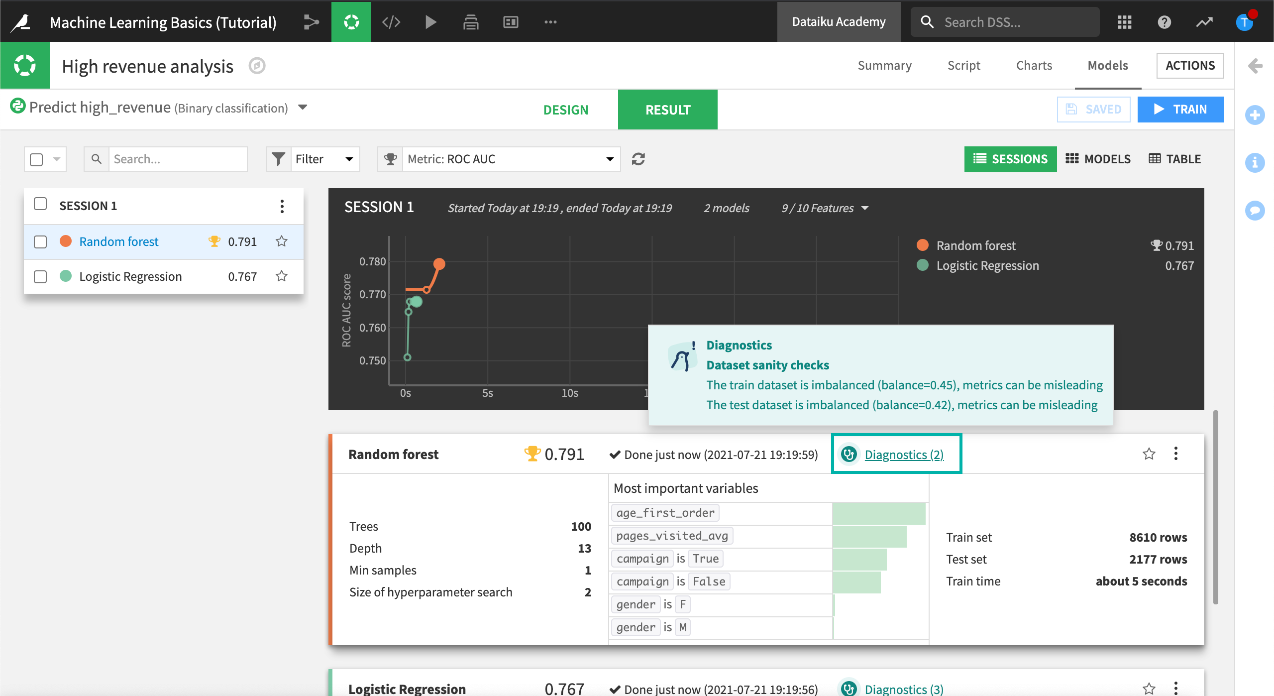
A few seconds later, DSS presents a summary of the results. By default, two classes of algorithms are used on the data:
a simple generalized linear model (logistic regression)
a more complex ensemble model (random forest)
While training the models, DSS runs visual ML diagnostics and displays the results in real time.
You can hover over the visual ML diagnostics as the models are trained to view any warnings.
Later, we’ll take a closer look at the model results including the ML diagnostics.
Our baseline model training session is complete. We’ll use these results for comparison as we iterate on our model and try to improve its performance.
In the next section, we’ll evaluate our baseline model using the model summary. The model summary includes the following information:
the type of model
a performance measure; here the Area Under the ROC Curve or AUC is displayed
a summary of the most important variables in predicting your target
The AUC measure is handy: the closer to 1, the better the model. Here the Random forest model seems to be the most accurate.
Click the Random forest model to view the main Results page for this specific model.
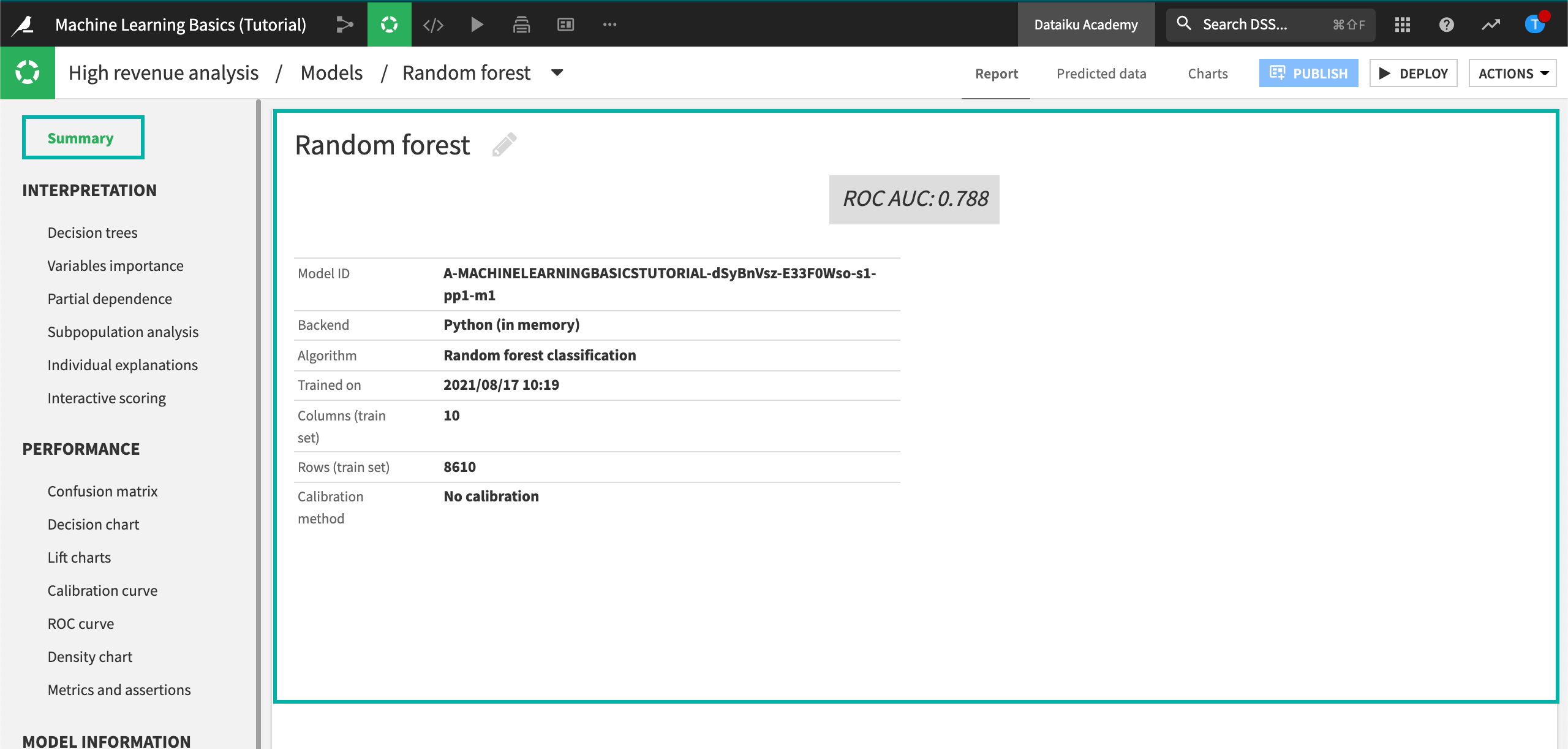
The Summary tab shows an ROC AUC value of approximately 0.791, which is pretty good for this type of application. Your actual figure might vary due to differences in how rows are randomly assigned to training and testing samples.
Note
You might find that your actual results are different from those shown. This is due to differences in how rows are randomly assigned to training and testing samples.
What’s next?
Congratulations! You have successfully built your first prediction model in DSS. There is a lot more to be done, however. In the next few lessons, you’ll dive deeper into how DSS can help you evaluate models like the one you have just built.