Hands-On Tutorial: Geo Join

Getting Started

In this tutorial, you’ll get hands-on practice with geospatial features by preparing and joining geospatial data to visualize credit card fraud activity on a map.

Prerequisites

To complete this tutorial, you’ll need the following:

• Access to a Dataiku DSS instance - version 10.0 or above.

If you don’t have a DSS 10 instance readily available, you can download the free edition. To get the free edition or start a hosted trial, visit the Dataiku website and click Get Started in the top right to see the different options.

Geospatial Features Used in This Tutorial

When you’ve completed this tutorial, you’ll have a better understanding of the following features:

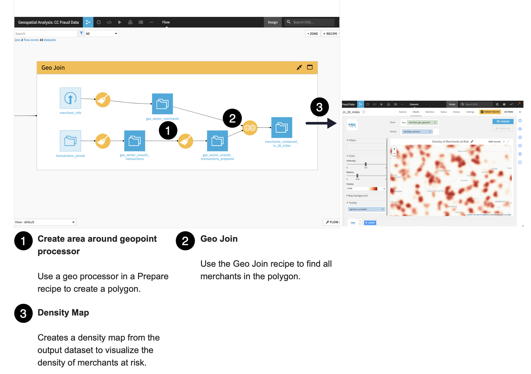
• Create area around geopoint processor

• Geo Join recipe

• Density map

What We’re Building

We’ll start by building out an existing project by creating new geographic features. Then, we’ll further build out the pipeline by joining on these features. Then we’ll create a density map that can be published to a dashboard.

How We’ll Build The Project

Our goal is to build a density map of merchants at risk of credit card fraud. To do this, we’ll create geographic features using the Prepare recipe and then join datasets using the Geo Join recipe.

We’ll limit our analysis to a specific merchant subsector, “gas”; and only those transactions that are flagged as fraudulent.

By creating geographic features, we’ll be able to focus on visualizing where the fraudulent transactions are occurring. This will allow us to identify “merchants at risk”. In other words, we’ll be able to visualize the density of merchants at risk of being targeted by the user of the stolen credit card.

Create and Explore the Project

In this section, we’ll create and explore the project. To create our project, we’ll open a tutorial that already has the input datasets we want to transform.

To open the tutorial:

• Sign in to your instance of Dataiku DSS.

• From the Dataiku DSS homepage, click on +New Project > DSS Tutorials > General Topics > Geospatial Analysis: CC Fraud Data.

Note

You can also download the starter project from this website and import it as a zip file.

Dataiku opens the Summary tab of the project, also known as the project homepage.

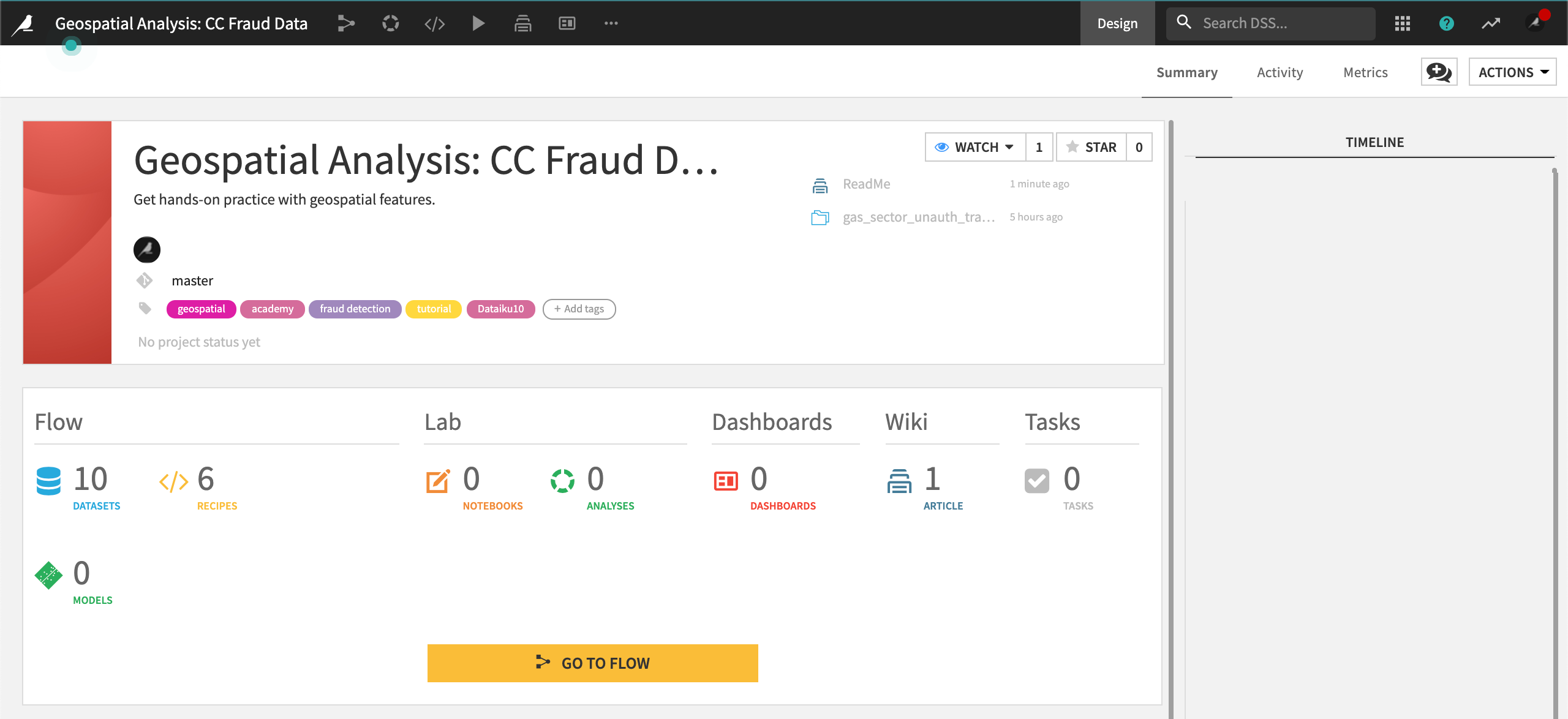
• Click Go To Flow.

• In the lower right corner, click Flow Actions, then select Build all.

• Click Build.

• Wait while Dataiku builds the Flow, then refresh your browser window.

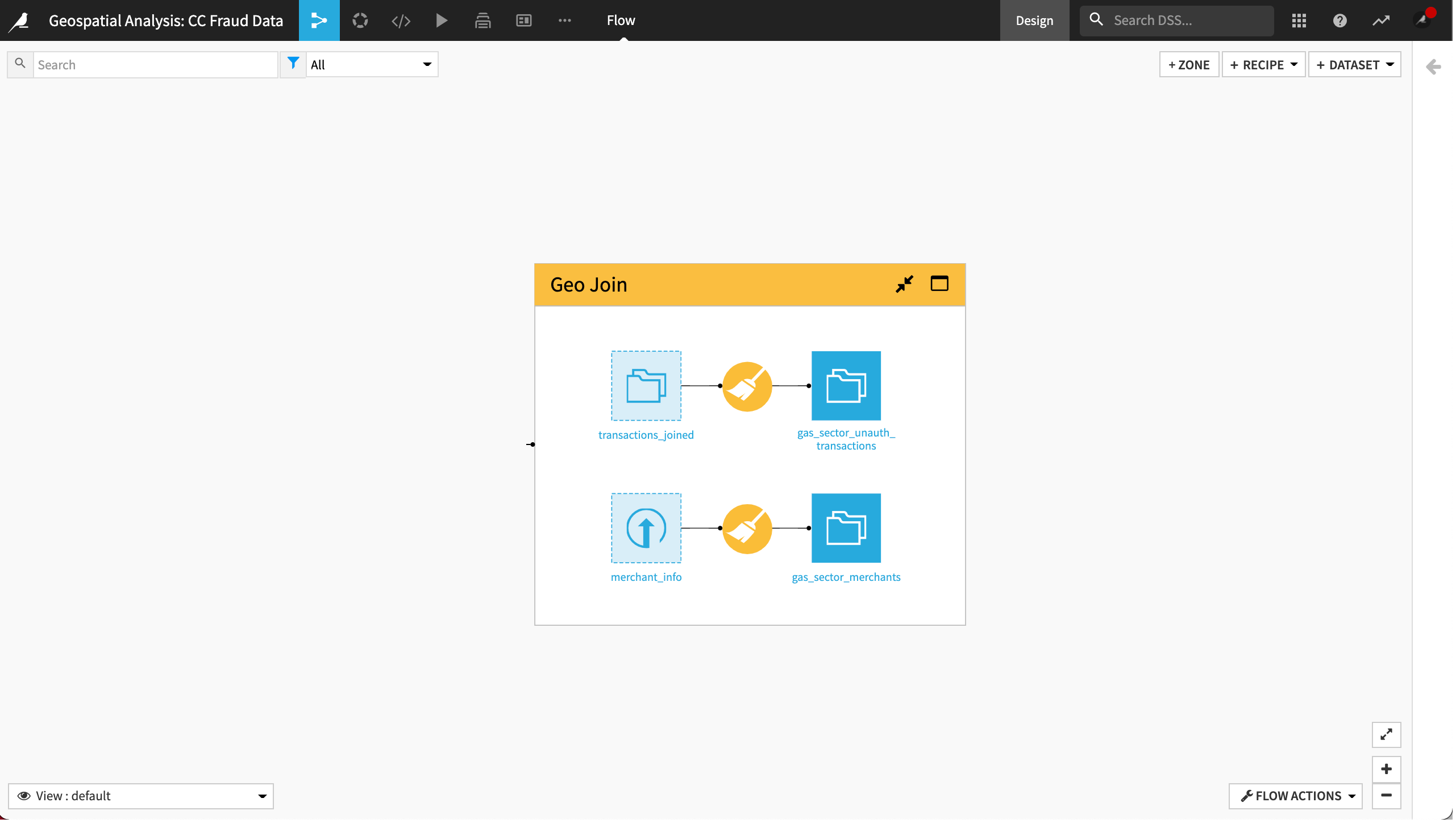
Explore the Flow

You’ll notice that the project contains more than one flow zone. For this lesson, we’ll focus on the following datasets in the Geo Join flow zone:

• gas_sector_unauth_transactions: This dataset has been prepared from transactions_joined and it contains the geopoints for all unauthorized transactions belonging to the gas merchant subsector. We’ll further prepare this dataset to create areas around the geopoints.

• gas_sector_merchants: This dataset has been prepared from merchants_info and it contains the geopoints for all merchants belonging to the gas merchant subsector.

Create Geographic Areas Around the Unauthorized Transactions

To visualize the number of merchants at risk around each unauthorized transaction, we’ll first need to create a geographic area around each unauthorized transaction’s geopoint. For this, we’ll use the Create area around geopoint processor in the Prepare recipe to operate on the existing geopoints in the dataset.

Let’s define a 20-mile geographic area.

• Go to the Flow.

• In the Geo Join flow zone, click the gas_sector_unauth_transactions dataset once to select it.

• Open the right-side panel, click Actions, then choose the Prepare recipe from Visual recipes.

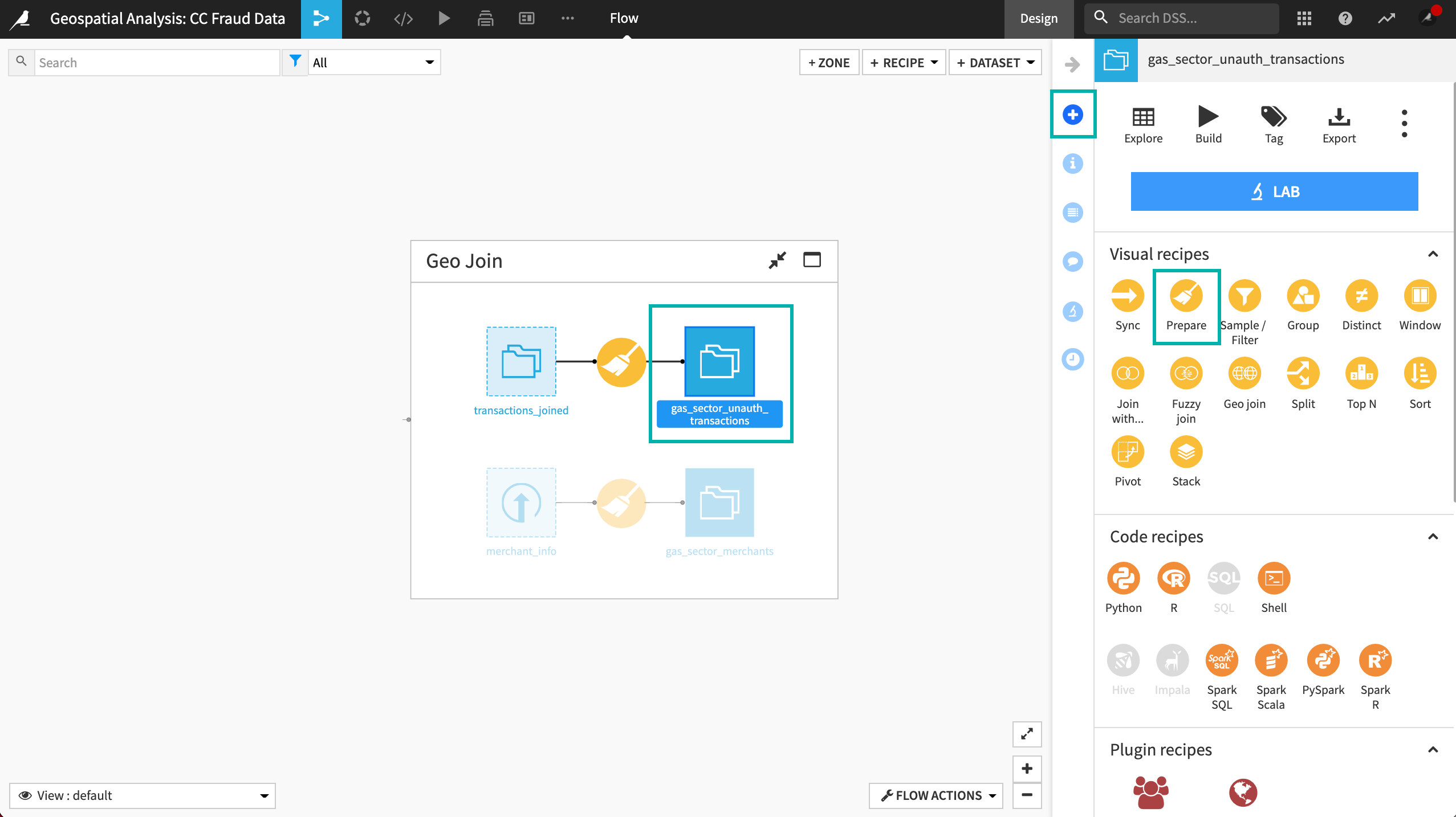
• Keep the default output dataset name and click Create Recipe.

Now, we’ll add a step to the script.

• In the Script, click + Add a New Step.

• In the processors library, search for geo and select Create area around geopoint.

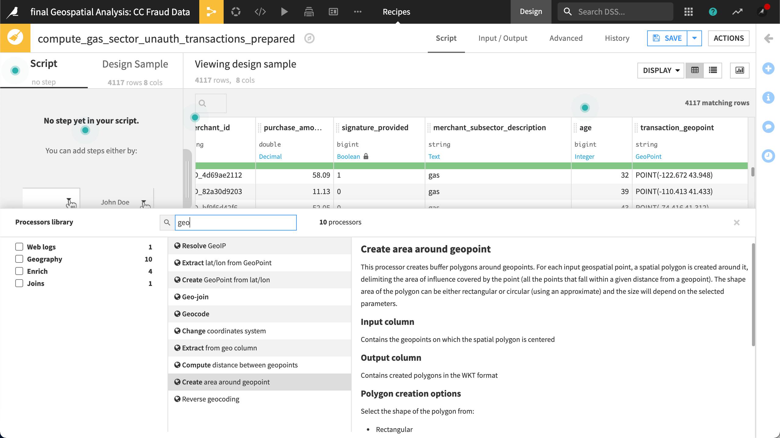
• Select transaction_geopoint as the Input column.

• Name the Output column 20_miles.

• Set the Shape to “Circle”.

• Define a Radius of 20, and a Distance unit of “Miles”.

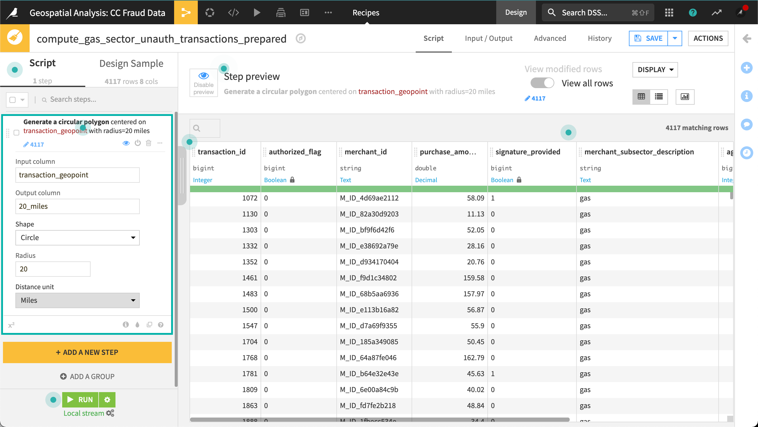
• Click Save and accept the schema update.

Throughout this tutorial, you can continue to update the schema when prompted.

Set Column Storage Type

Dataiku has inferred the storage type of our new geographic area column as “string”. Let’s set the storage type of the column to “Geometry” to match the values in the column.

• At the top of the 20_miles column, click the storage type, string, and select Geometry / Geography from the drop-down list.

• Likewise, set the storage type of transactions_geopoint to Geo Point.

• Save and Run the recipe.

• Update the schema when prompted.

• Explore the output dataset.

Now that we have defined geographic areas around the geopoints of unauthorized transactions, we can use the Geo Join recipe to map merchants to the areas.

Join Two Datasets Using Geospatial Data

In this section, we’ll create a dataset that includes all of the merchants located within each 20-mile geographic area. Later, we’ll create a chart to visualize the density of the merchants within these areas.

To create our dataset, we’ll use the Geo Join recipe.

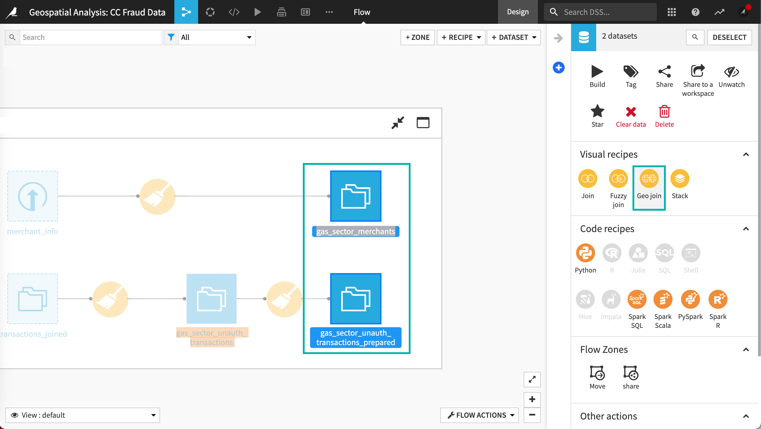
• Return to the Flow.

• In the Geo Join flow zone, click the newly created gas_sector_unauth_transactions_prepared dataset to select it.

• Hold down the Shift key then click the gas_sector_merchants dataset to select it, too.

• Open the right-side panel and choose the Geo join recipe from Visual recipes.

Dataiku displays the New geojoin recipe window.

• Name the output dataset merchants_contained_in_20_miles instead of the default name.

Your recipe window should look like this:

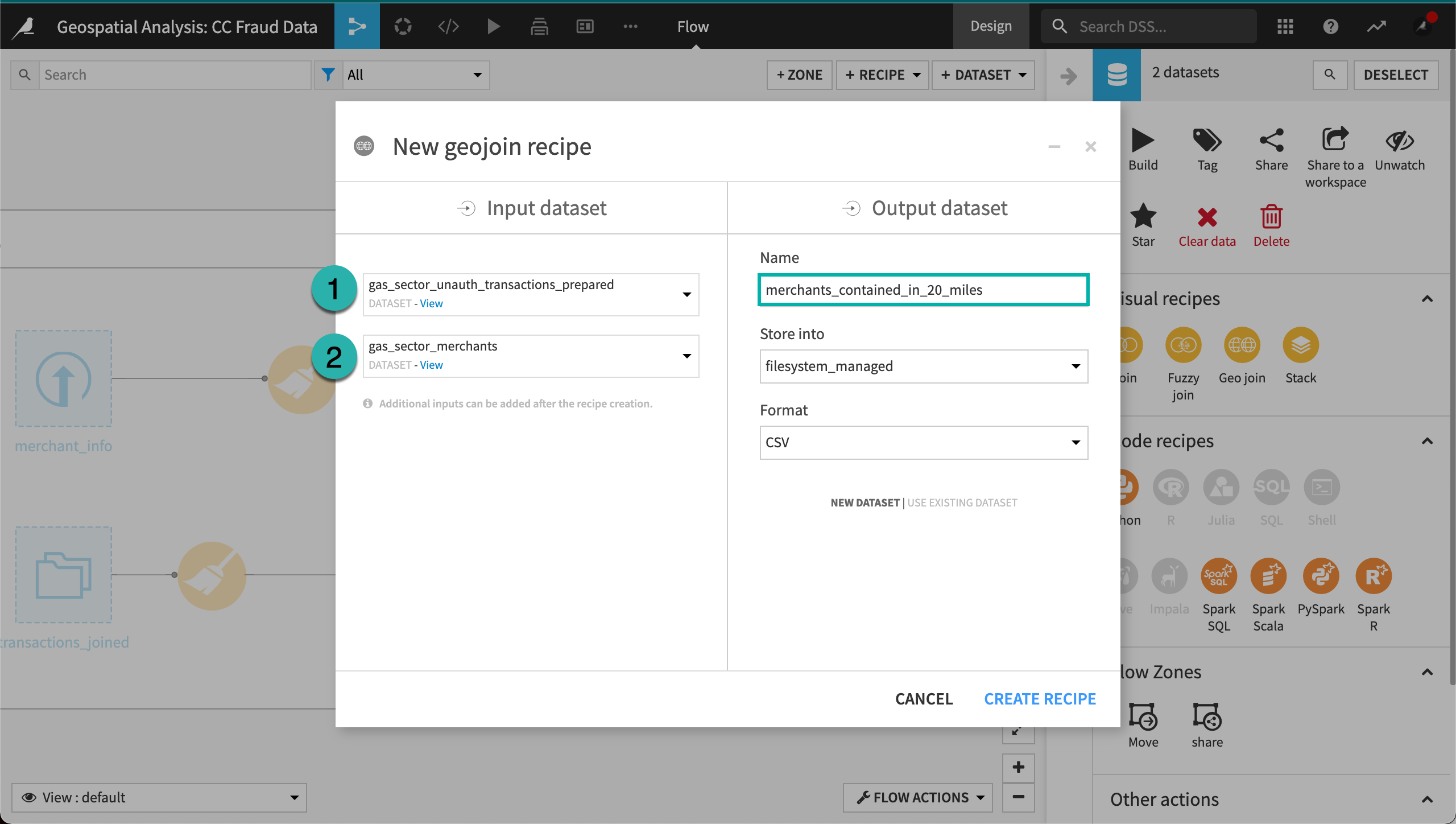
• Click Create Recipe.

Note

If Dataiku displays “No available join columns”, return to your input datasets and ensure that the storage types of the geospatial columns (transaction_geopoint, merchant_gas_geopoint, and geometry) are set to type Geo Point or Geometry / Geography, as applicable.

Dataiku displays the Join step of the recipe. By default, Dataiku selects available geospatial columns to use for the join and specifies a join condition. Here, Dataiku has selected the transaction_geopoint column from our left dataset as the join key. However, we’ll perform this join using the polygon we created.

Let’s configure the Join conditions.

• Click transaction_geopoint to display the Join conditions.

Dataiku displays the Join window.

Let’s keep the default Left join type and the Match when all the following conditions are satisfied selection.

• Click transaction_geopoint again to open the Join conditions window.

• Set “Column from” to 20_miles and the join condition to Contains.

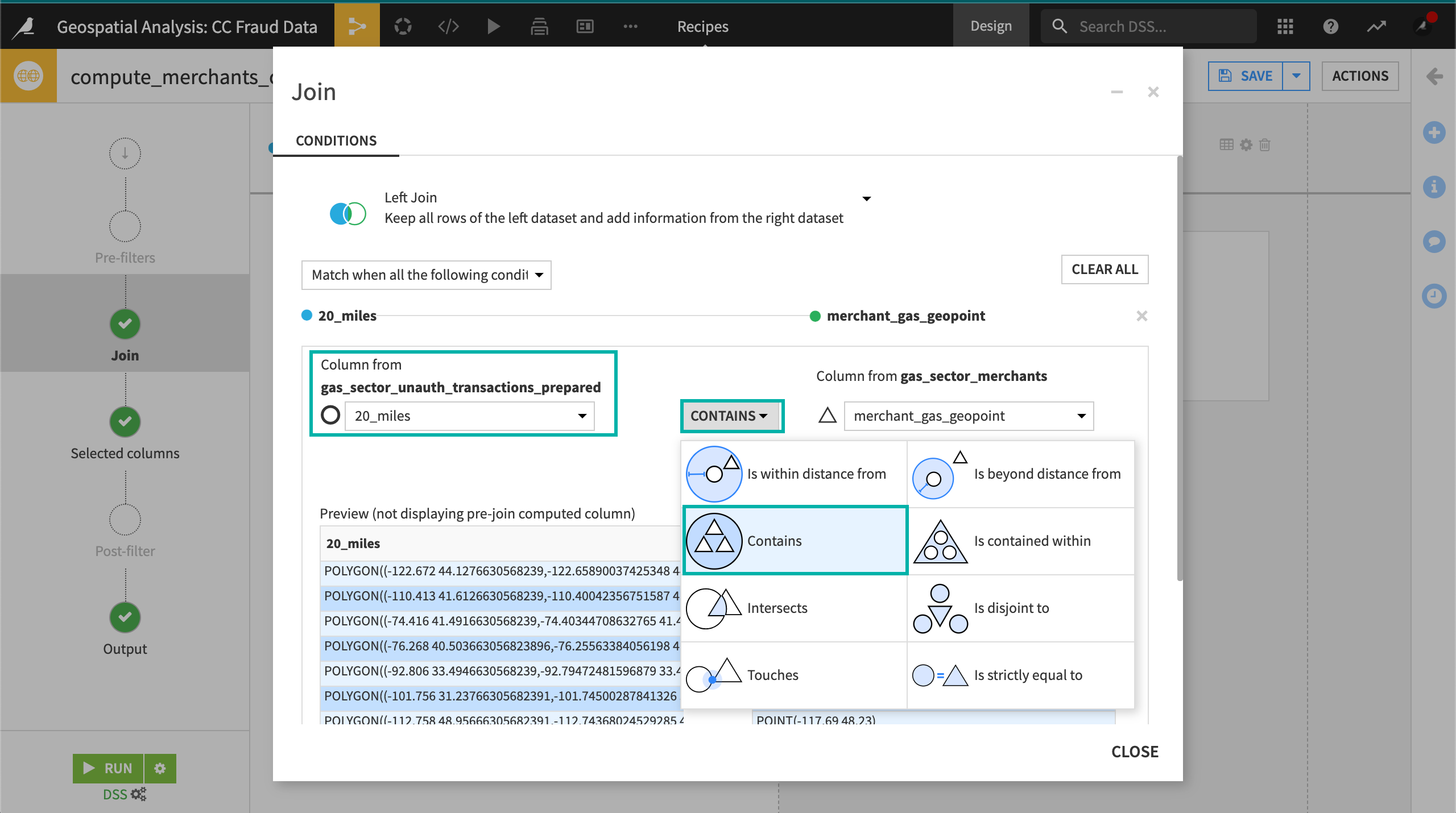
• Close the Join conditions window.

Let’s configure the columns in the output dataset, removing any that we don’t need.

• Go to the Selected columns step.

• In gas_sector_unauth_transactions, remove the transaction_geopoint column.

• In gas_sector_merchants, remove the subsector_description column.

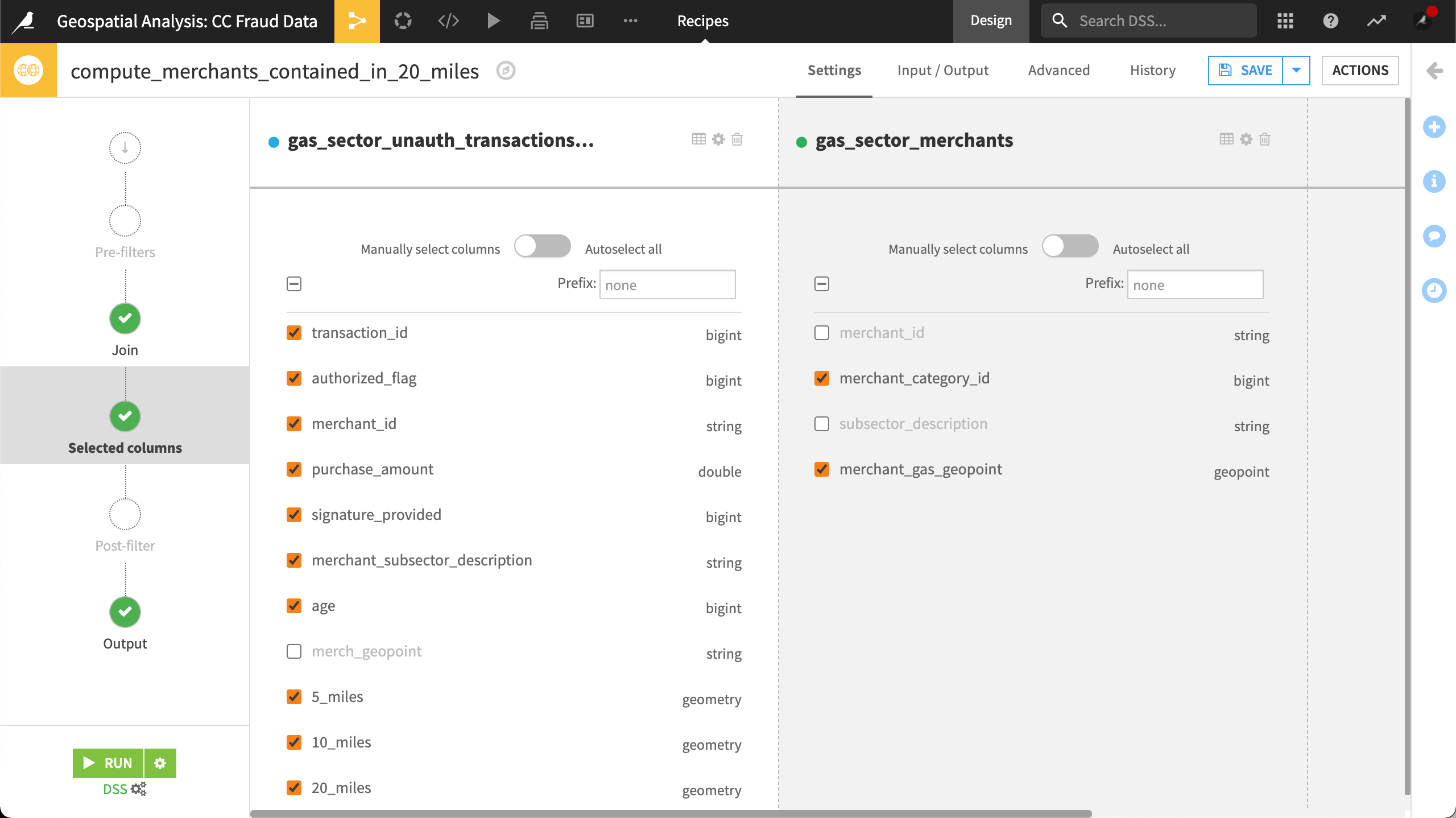
• Save and Run the recipe.

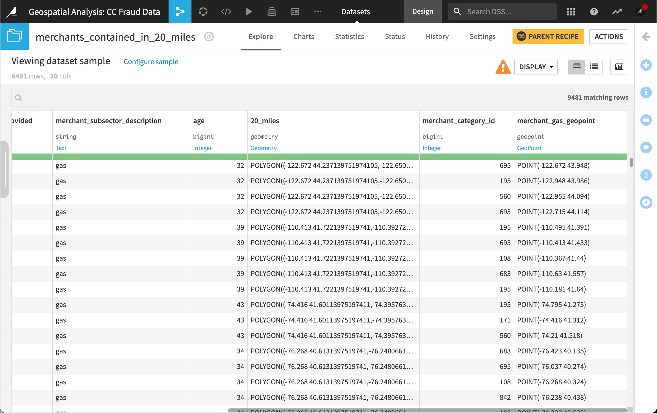
• Explore the output dataset.

Create a Density Map

In this section, we’ll build a type of chart known as a density map. The map takes as an input a column containing geo points and represents them in the form of a heat map. We can customize our map by selecting a color palette, configuring the intensity, and setting the radius of the circles for each point.

While a density map and scatter map may seem similar, we’ll soon discover how valuable a density map can be when plotting a large set of points on a map. Since the density map allows us to show where geopoints are concentrated on a map, we can quickly understand where, on a map, there are areas with a lot of points, or where there are areas with very few points.

Let’s create our map!

• Return to the Flow.

• Open the merchants_contained_in_20_miles dataset.

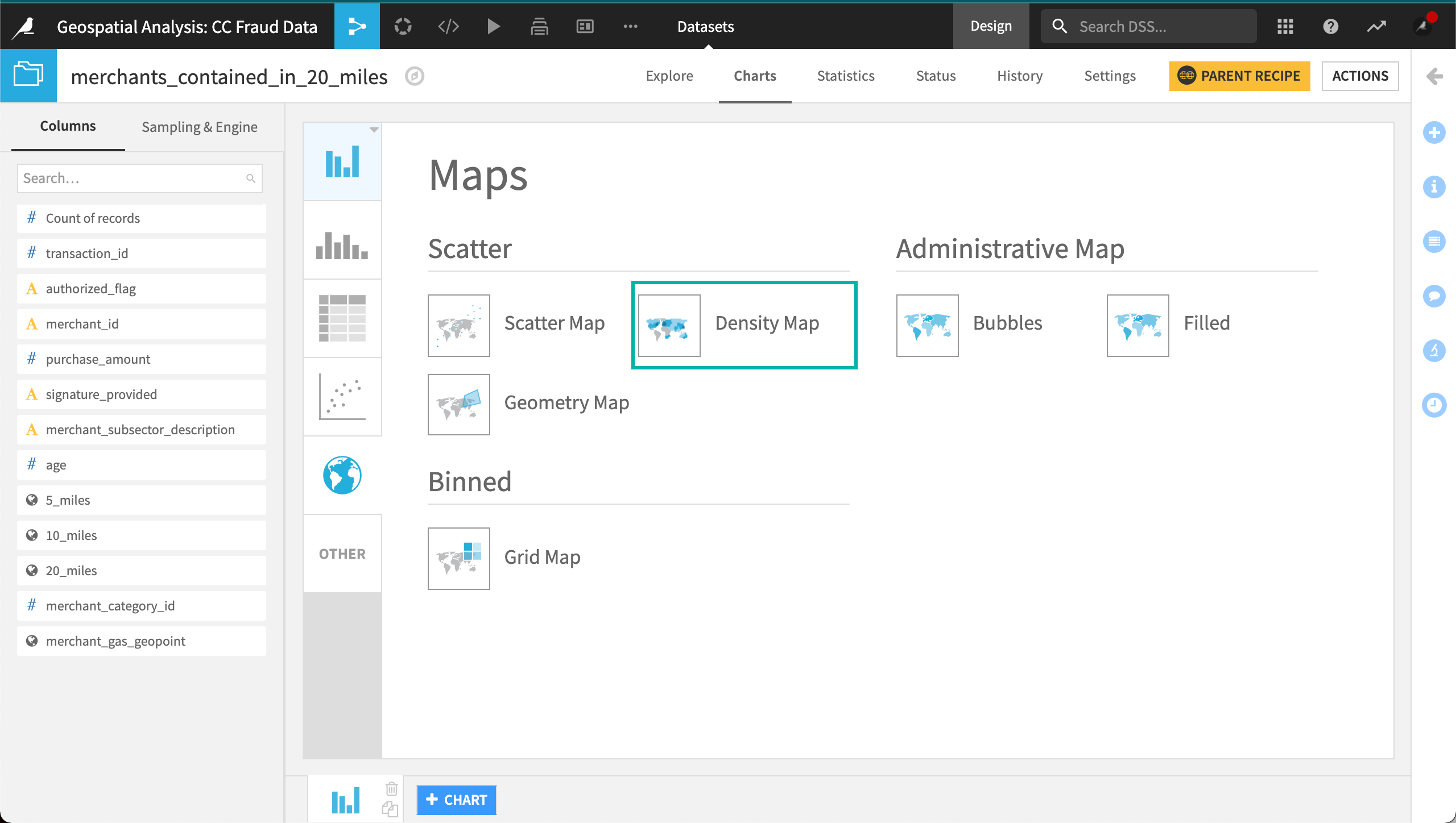
• Click on the Charts tab.

• Click the Chart symbol in the upper left to view the chart options and types.

• Choose the Map chart type, then select the Density Map.

• From the Columns panel on the left, drag and drop merchant_gas_geopoint to Geo.

• Drag and drop purchase_amount to Details to set the heatmap’s intensity.

Let’s configure the radius of our circles, the color palette, and add a tooltip.

• Open the Color panel, then set the Radius to approximately “0.25”.

• Select OrRd from the Palette.

• Open the Tooltip panel, then drag and drop the signature_provided column to set the tooltip.

You can zoom in on the map to see more details.

• Edit the title of the chart to Density of Merchants at Risk.

Here’s what the chart looks like when zoomed in.

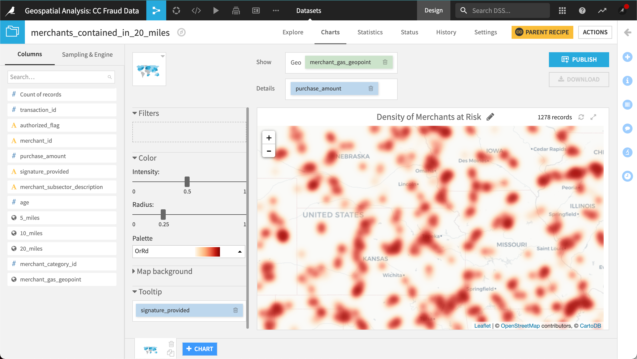
Using our Density Map, we can now visualize the geographic relationship between merchant location and transactions flagged as fraudulent. More specifically, we can visualize the concentration of merchants at risk in each geographic area.