Hands-On: Scoring Data
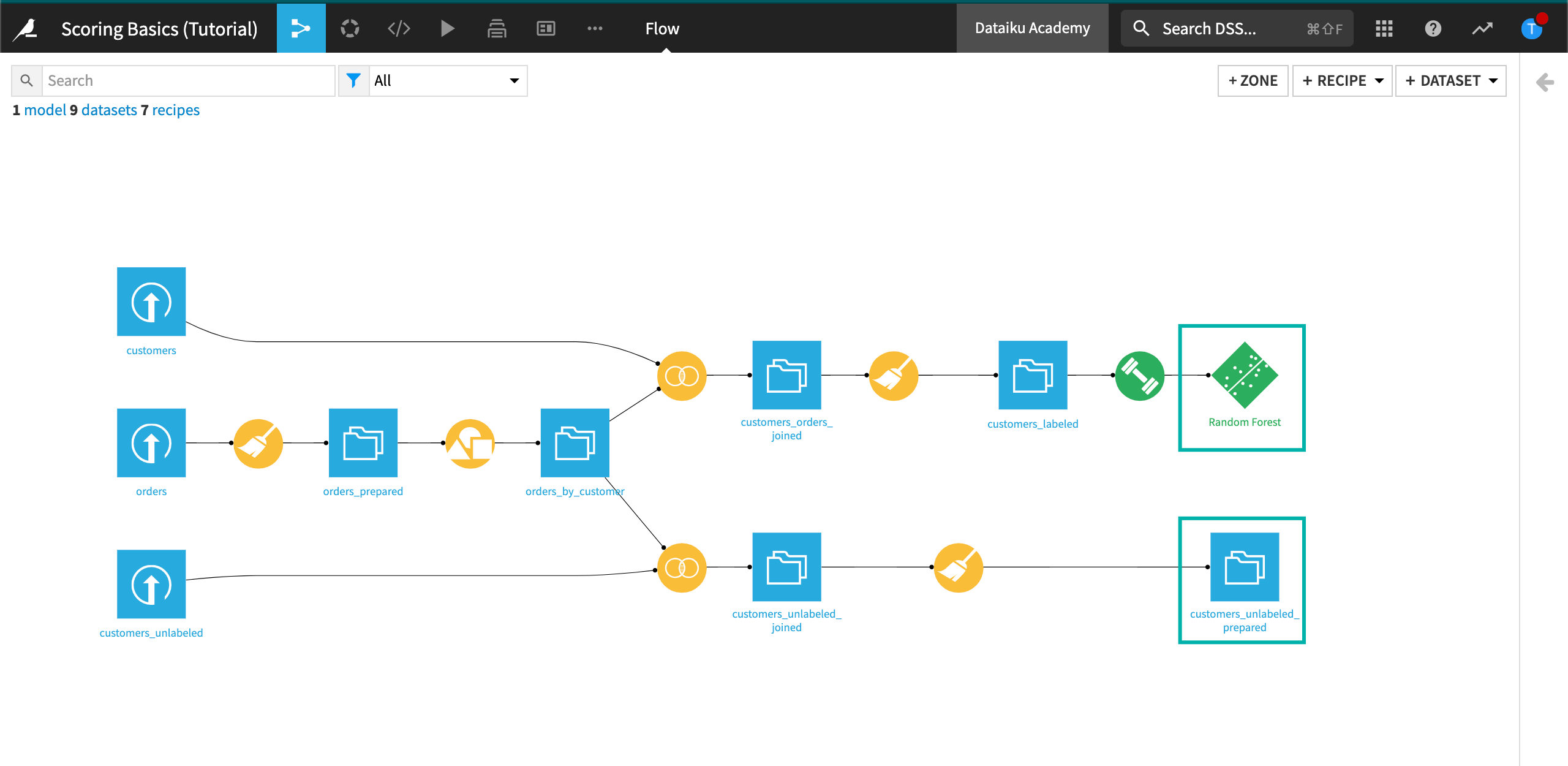
In the last hands-on lesson, we deployed our best-performing model from the Lab to the Flow. Our objective now is to use that same model (Random Forest) and apply it to a dataset of new customers (customers_unlabeled_prepared).
Active Version of the Model
If you choose the model deployed in the Flow, you will be redirected to a view, similar to the Models one from your previous analysis bench, but focusing only on the model you chose to deploy (the random forest):
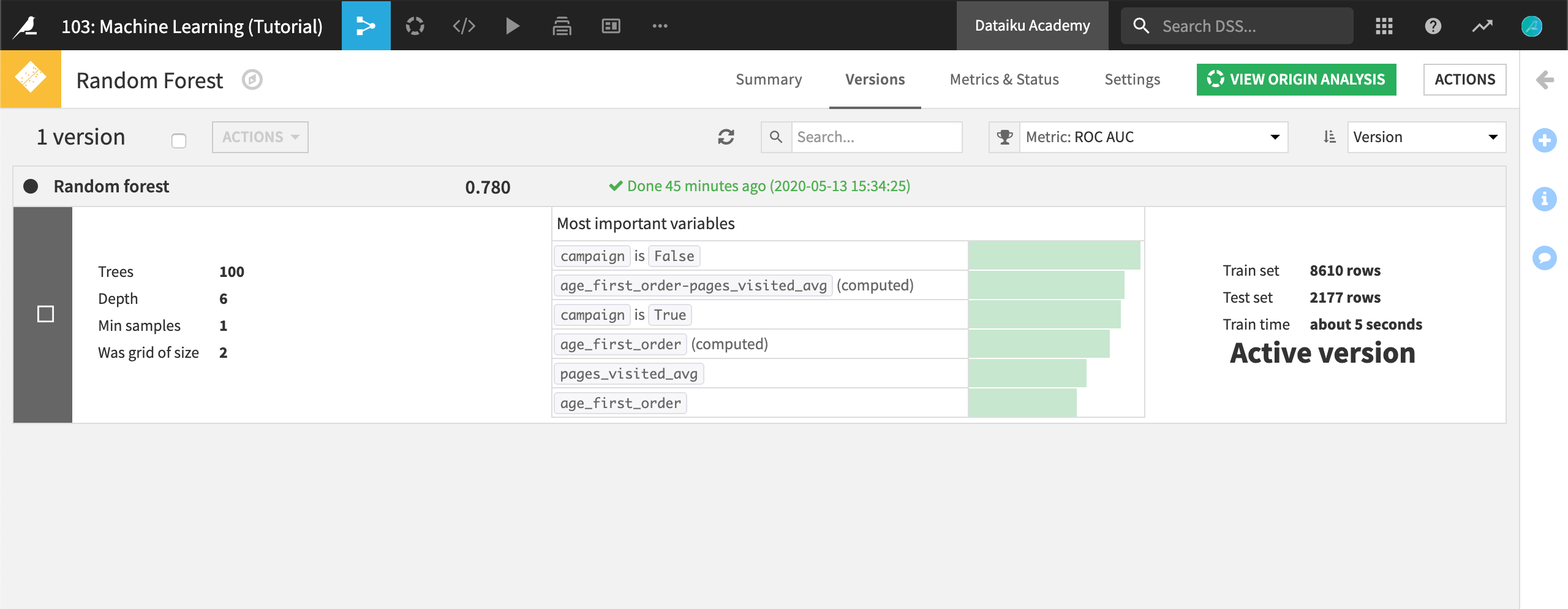
Without going into too much detail in this tutorial, notice that the model is marked as the Active version. If your data were to evolve over time (which is very likely in real life!), you could train your model again by clicking on Actions and then Retrain from this screen. In this case, new versions of the models would be available, and you would be able to select which version of the model you’d like to use.
Go back to the Flow and click on the model output icon.
You should see a Retrain button close to the Open one. This is a shortcut to the function described above: you can update the model with new training data, and activate a new version.
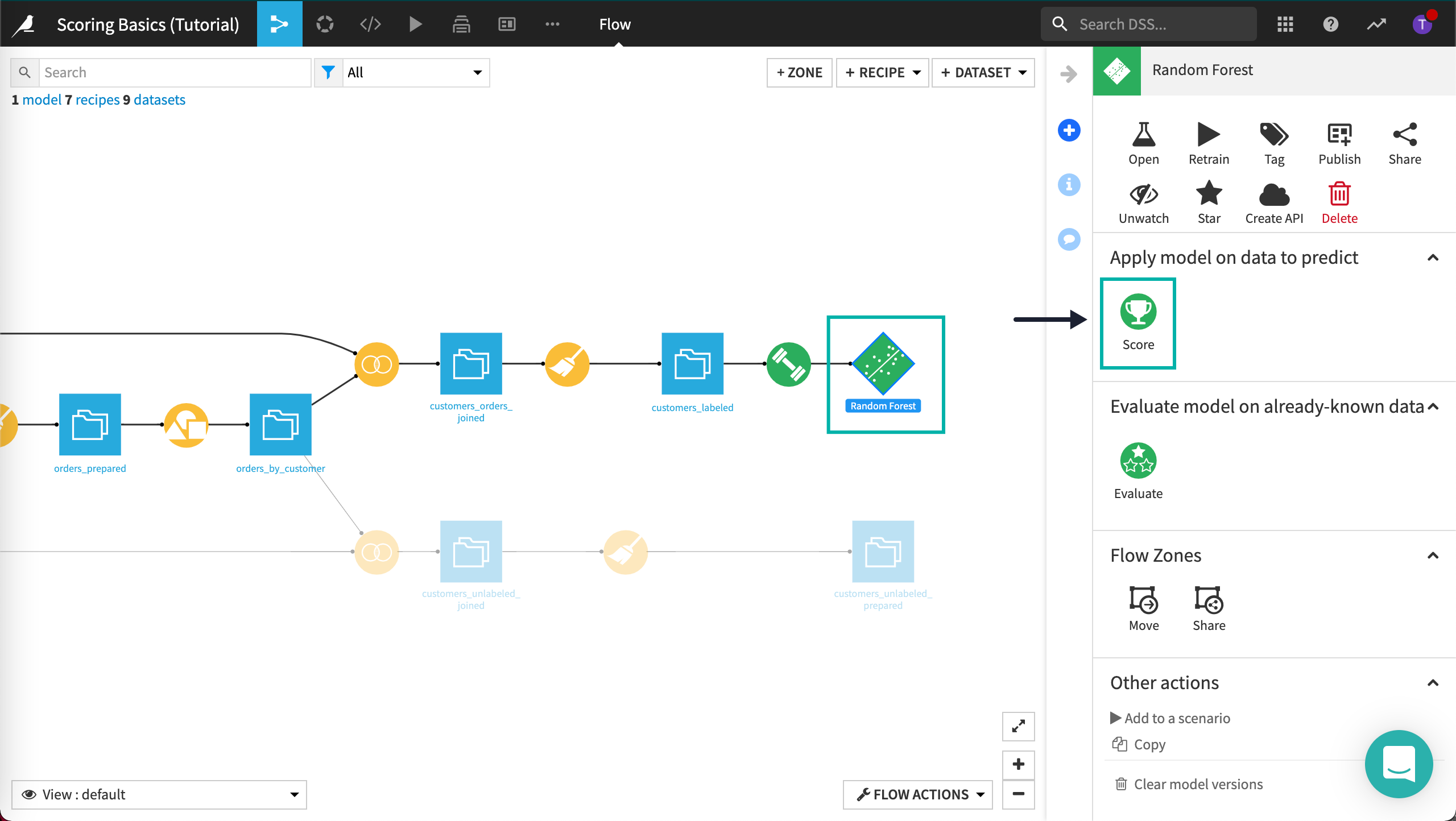
The Score Recipe
Finally, the Score icon is the one we are looking for to apply the model to new data.
Click the deployed model in the Flow to select it.
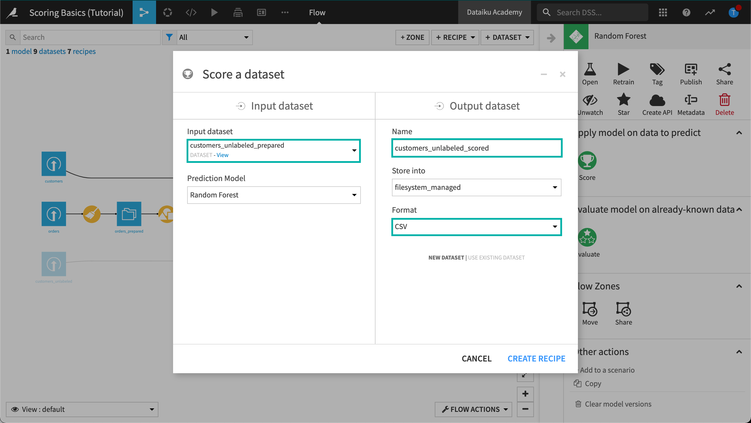
Configure the input and output datasets as follows:
Set the input dataset to customers_unlabeled_prepared.
Name the output dataset
customers_unlabeled_scored.Select the Format where you want to store the results into, such as “CSV”.
Click Create Recipe.
You are now in the Scoring recipe.
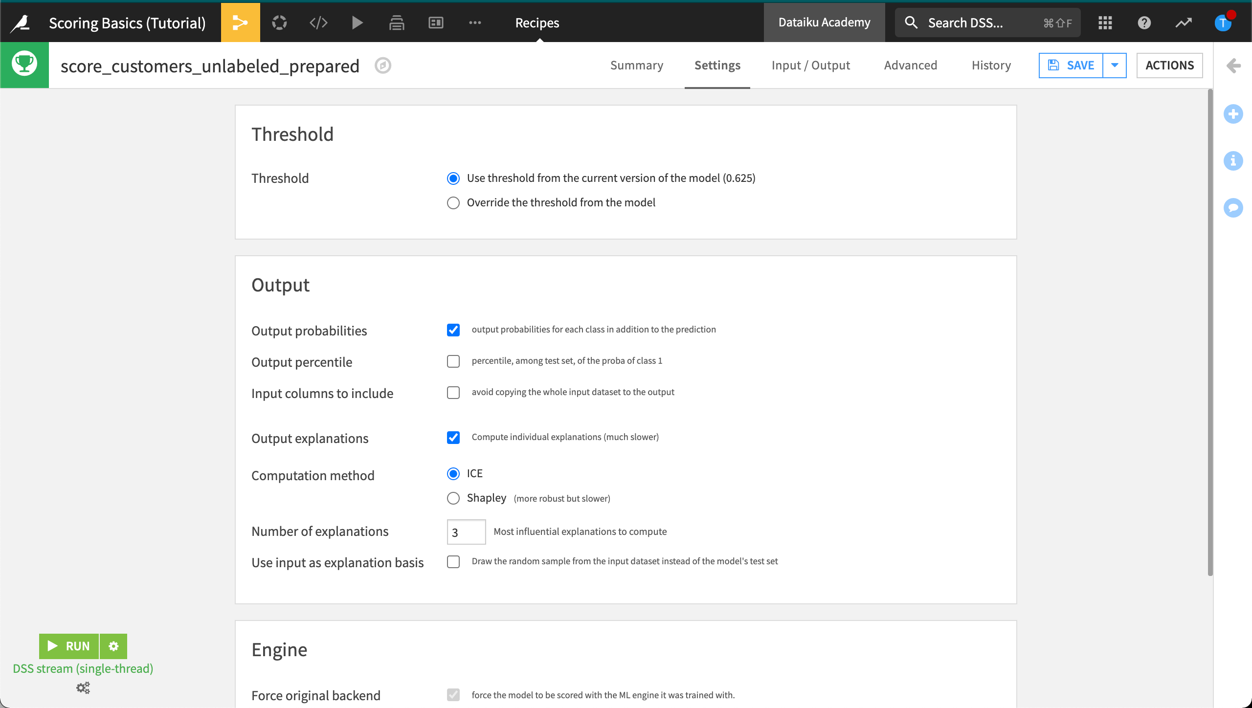
As discussed in the Machine Learning Basics course, the threshold is the optimal value computed to maximize a given metric. In our case, it was set to 0.625. Rows with probability values above the threshold will be classified as high value, below as low value.
If you would like to return individual explanations of the prediction for each row in the customers_unlabeled_prepared dataset:
Click the checkbox for “Output explanations”. This action enables the “Force original backend” option so that the model can be scored with the same machine learning engine used during its training. Enabling the “Output explanations” checkbox also brings up some additional parameters:
For the “Computation method”, keep the default “ICE”.
For the “Number of explanations”, keep the default
3. This returns the contributions of the three most influential features for each row.
Finally, click the Run button at the bottom left to score the dataset.
Accept the schema update, if prompted, by clicking Update Schema.
A few seconds later, you should see Job succeeded.
Return to the Flow.
To recap, you:
Started from the “historic data”.
Applied a training recipe.
Created a trained model.
Applied the model to get the scores on the unlabeled dataset.
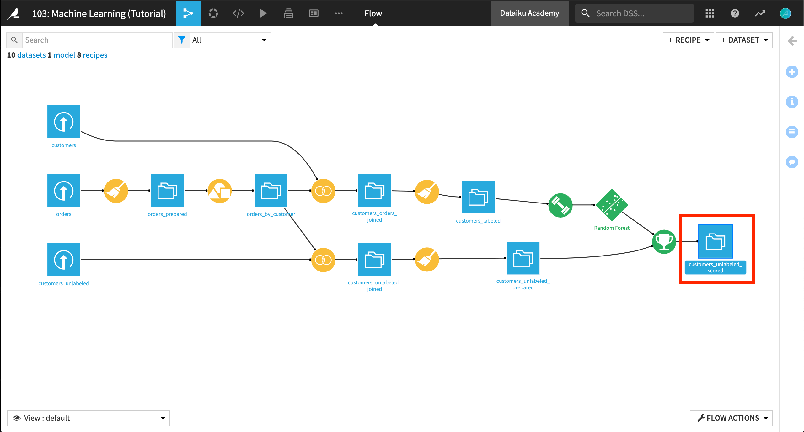
Inspect the Scored Results
We’re almost done! Open the customers_unlabeled_scored dataset to see how the scored results look.
Four new columns have been added to the dataset:
proba_False
proba_True
prediction
explanations (as requested in the Scoring recipe)
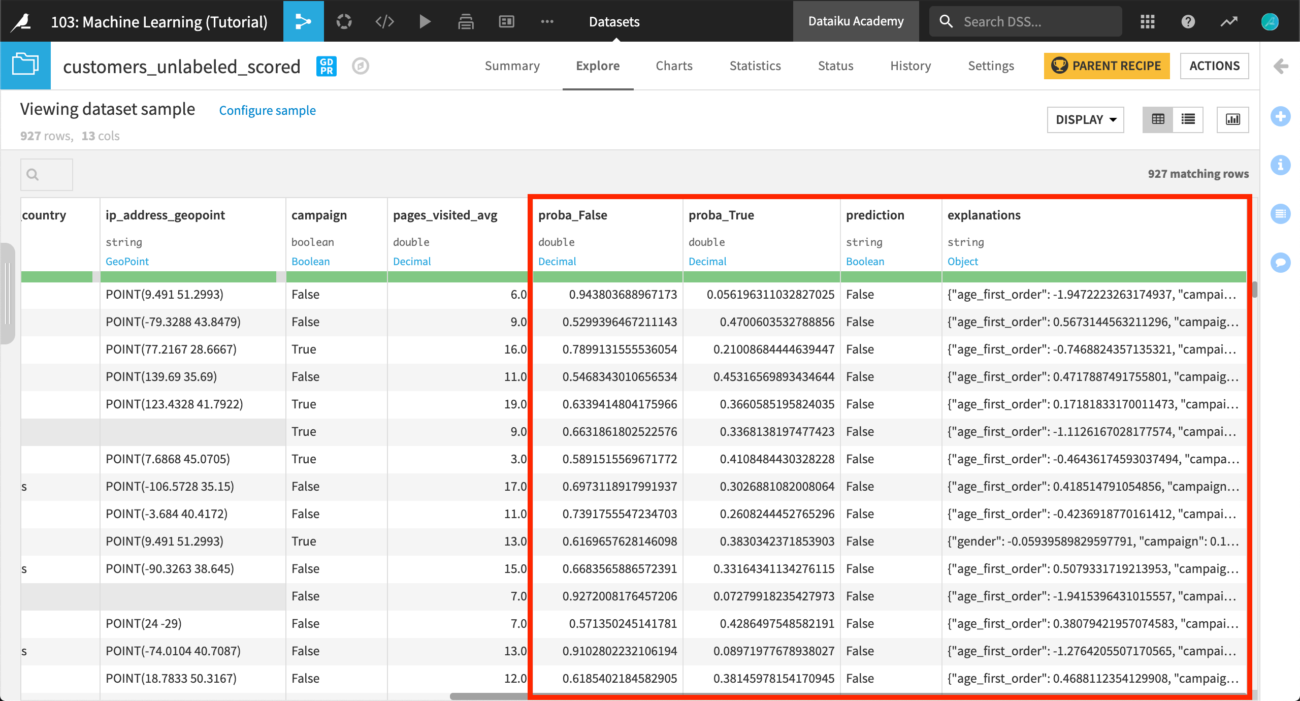
The two “proba” columns are of particular interest. The model provides two probabilities, i.e. a value between 0 and 1, measuring the likelihood to become a high value customer (proba_True), and the opposite likelihood to not become a high value customer (proba_False).
The prediction column is the decision based on the probability and the threshold value of the scoring recipe. Whenever the column proba_True is above the threshold value (in this case, 0.625), then DSS will label that prediction “True”.
The explanations column contains a JSON object with features as keys and their positive or negative influences as values. For example, the highlighted row in the following figure shows the three most influential features (age_first_order, campaign, and pages_visited_avg) for this row and their corresponding contributions to the prediction outcome.
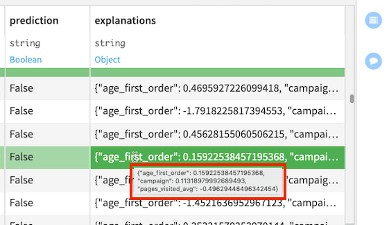
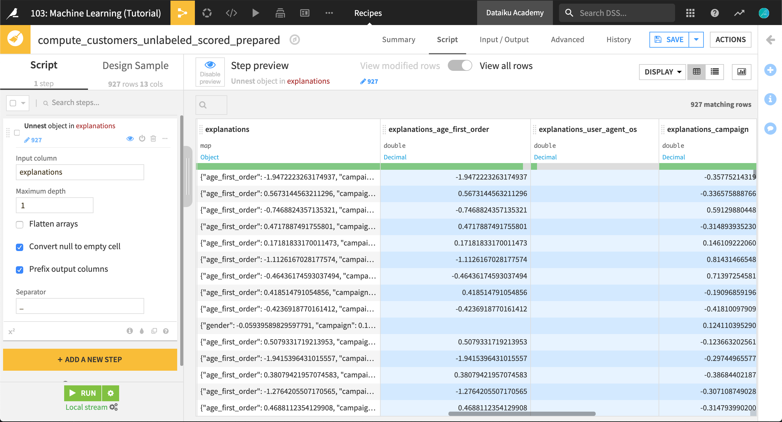
In order to more easily work with the JSON data in this column, you can create a Prepare recipe on the customers_unlabeled_scored dataset. In the recipe, apply the Unnest object (flatten JSON) processor to the explanations column.
To learn more about individual prediction explanations, see the reference documentation.
Learn More
That’s it! You now know enough to build your first predictive model, analyze its results, and deploy it. These are the first steps towards a more complex application. Great job!