Introduction to Reinforcement Learning
The past few years have witnessed breakthroughs in reinforcement learning (RL). From the first successful use of RL by a deep learning model for learning a policy from pixel input in 2013 to the OpenAI Dexterity program in 2019, we live in an exciting moment in RL research.
In this first article, you’ll learn about:
The meaning of RL and the core concepts within this technique
The three approaches to RL
The concept of deep reinforcement learning
What is Reinforcement Learning
The main idea behind Reinforcement Learning (RL) is that an agent will interact with its environment, learn from it, perform actions, and receive rewards as feedback for these actions.

As humans, learning from our interactions with the environment comes naturally. Imagine you’re a child in a living room. You see a fireplace and approach it.
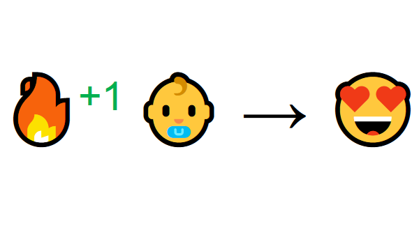
The fireplace feels warm; therefore, you feel good (Positive Reward +1). You understand that fire is a positive thing.
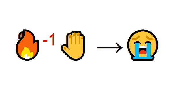
But then you try to touch the fire. Ouch! It burns your hand (Negative reward -1).
You’ve just understood that fire is positive when you are a sufficient distance away because it produces warmth, but get too close, and it burns.
This example illustrates how humans learn — through interaction. Reinforcement Learning is just a computational approach to learning from action.
Core Concepts of Reinforcement Learning
To discuss the core concepts of RL, we will focus on describing:
The RL process
Tasks within RL — Episodic or Continuing Tasks
Learning methods — Monte Carlo vs. TD Learning
The Exploration/Exploitation Trade-off
The Reinforcement Learning Process
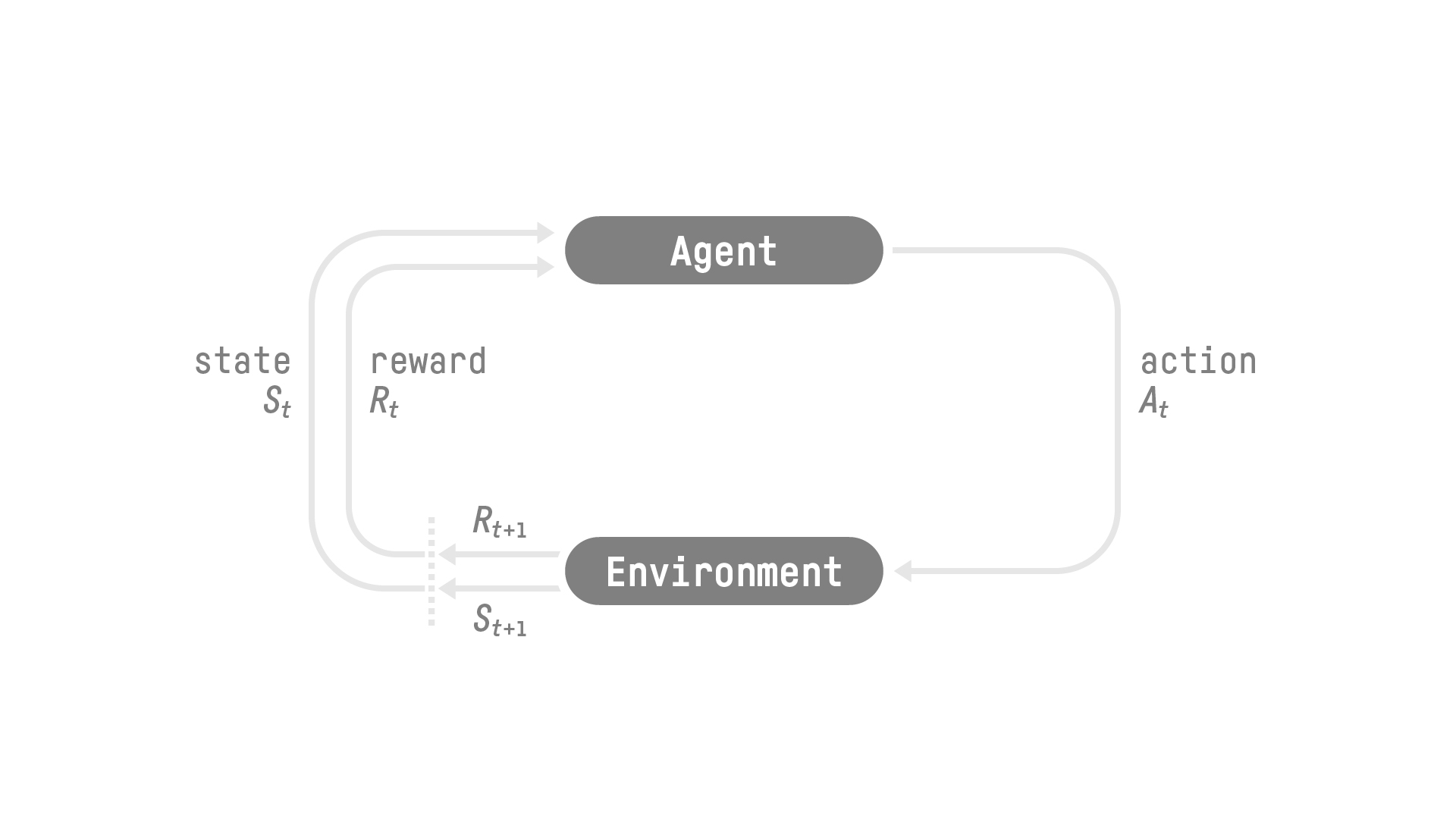
The Reinforcement Learning (RL) process can be modeled as a loop that works like this:
Now, let’s imagine an agent learning to play a platform game. The RL process looks like this:
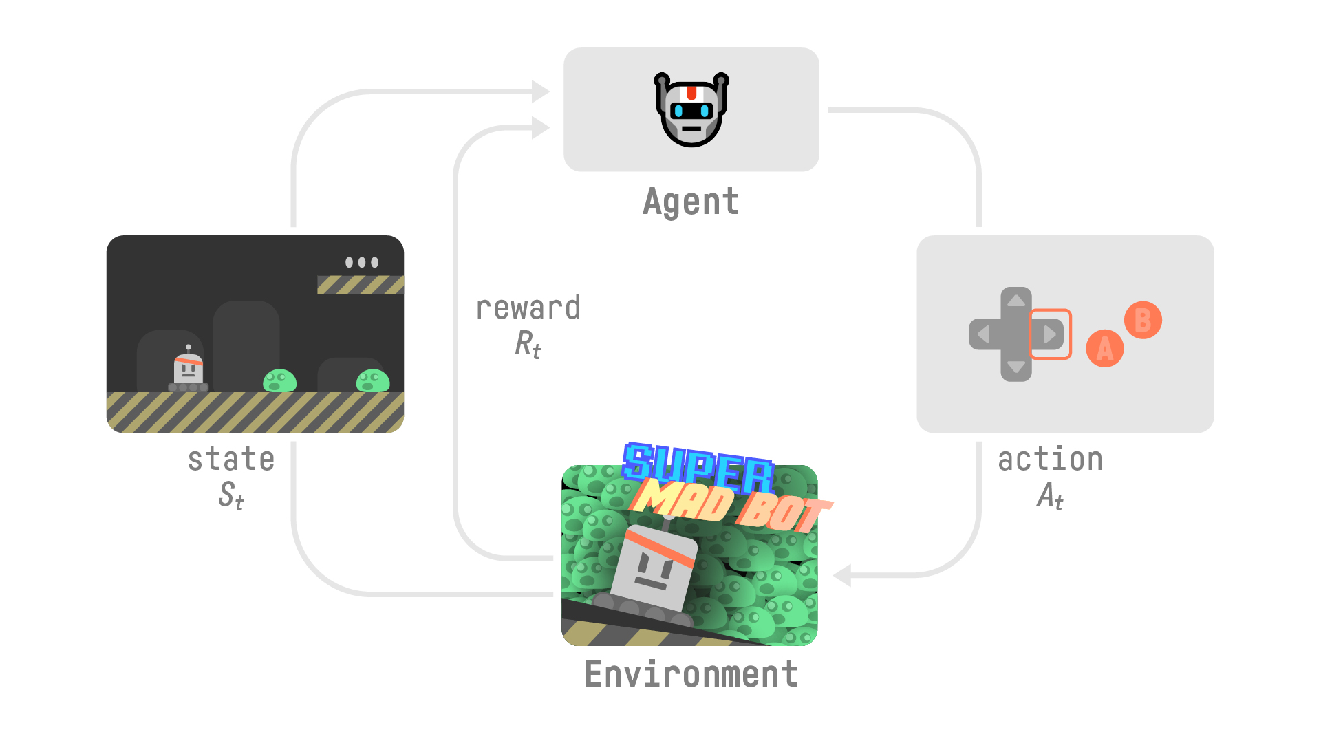
Our agent receives state \(S_0\) from the environment — we receive the first frame of our game (environment).
Based on the state \(S_0\), the agent takes an action \(A_0\) — our agent will move to the right.
The environment transitions to a new state \(S_1\).
Give a reward \(R_1\) to the agent — we’re not dead (Positive Reward +1).
This RL loop outputs a sequence of state, action, and reward. The goal of the agent is to maximize the expected cumulative reward.
The Central Idea of the Reward Hypothesis
Why is the goal of the agent to maximize the expected cumulative reward? Well, because reinforcement learning is based on the idea of the reward hypothesis.
The reward hypothesis means that all goals can be described as the maximization of the expected cumulative reward. Hence, to have the best behavior, we must maximize the expected cumulative reward.
The cumulative reward at each time step t can be written as:

\(G_t\) equals the sum of all rewards at each time step t.
This equation is equivalent to (where T is the terminal state):
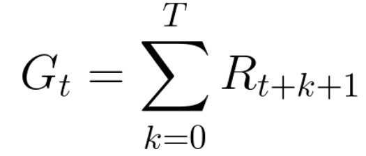
However, in reality, we can’t just add rewards this way. The rewards that come sooner (at the beginning of the game) have a higher chance of happening since they are more predictable than the long-term future rewards.
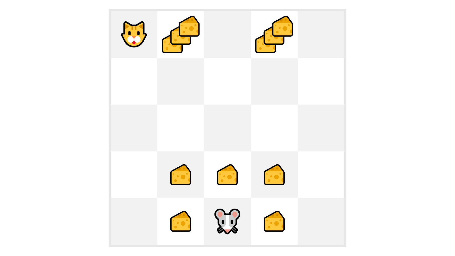
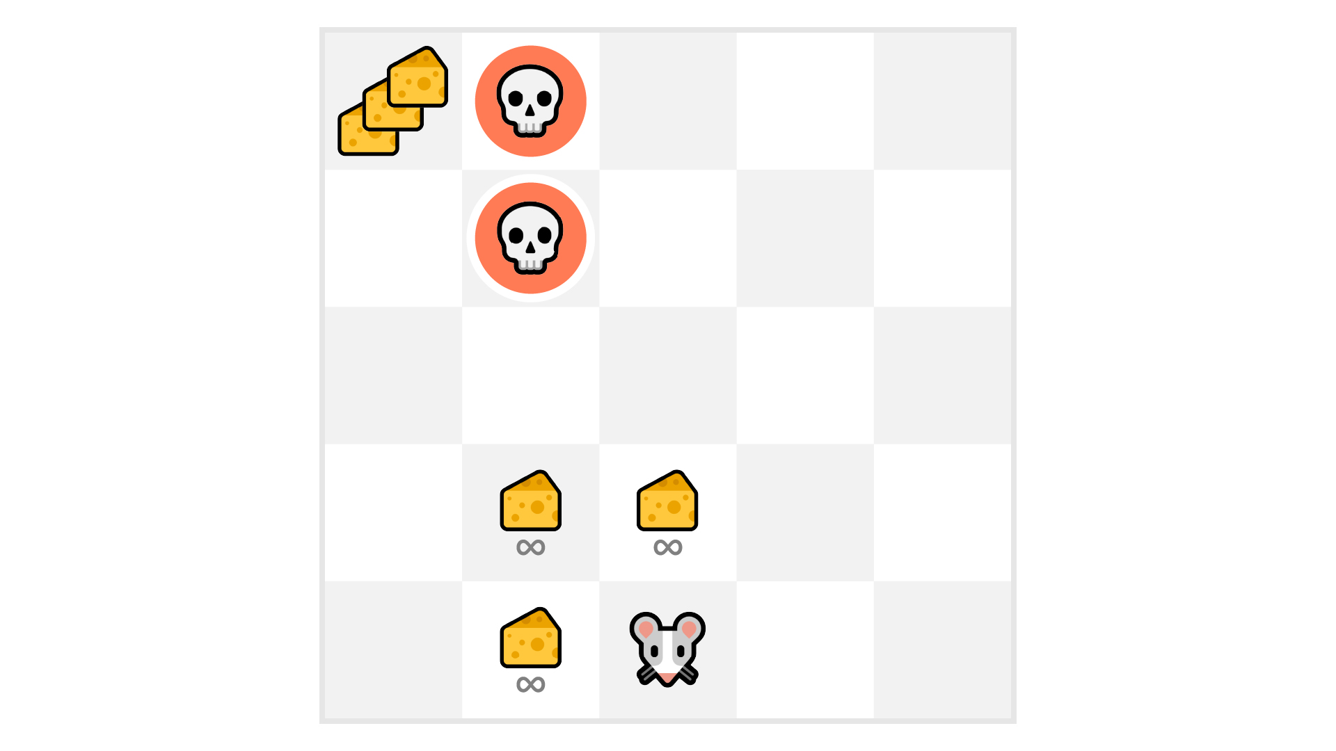
As an example, consider that your agent is a small mouse, and your opponent is the cat (as shown in the previous figure). Your goal is to eat the maximum amount of cheese before being eaten by the cat.
As we can see in the figure, your agent is more likely to eat the cheese within its immediate vicinity than the cheese farther away (and close to the cat). The closer the mouse gets to the cat, the more dangerous things become.
Consequently, though the reward near the cat is bigger (more cheese), it will be discounted, because it is unlikely to be attained.
To discount rewards, we proceed by defining a discount rate, gamma (𝜸), with values between 0 and 1.
The larger the value of gamma, the smaller the discount. Thus, the learning agent cares more about the long term reward.
On the other hand, the smaller the value of gamma, the bigger the discount. Thus, our agent cares more about the short term reward (the nearest cheese).
Consequently, the discounted cumulative expected reward is:
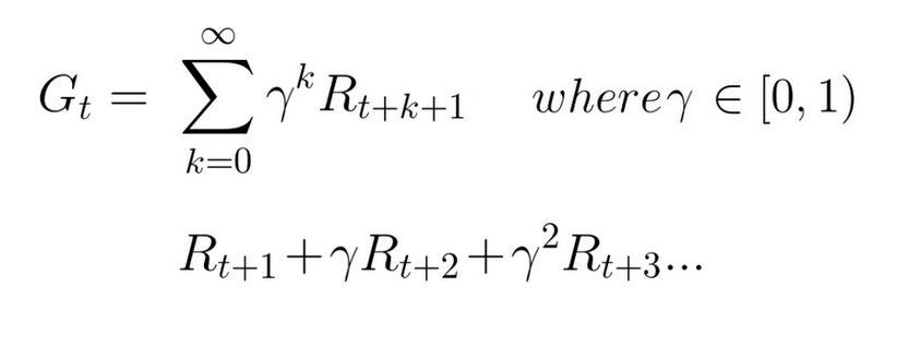
Simply put, each reward will be discounted by gamma to the exponent of the time step. As the time step increases, the cat gets closer to us, so the future reward is less and less likely to happen.
Episodic or Continuing Tasks
A task is an instance of a reinforcement learning problem. A task can either be episodic or continuous.
Episodic Task
In this case, we have a starting point and an ending point (a terminal state T), thereby creating an episode: a list of states, actions, rewards, and new states.

For instance, think about any video game. An episode begins at the launch of a new level and ends when you’re killed, or you’ve reached the end of the level.
Continuous Task
These are tasks that continue forever (no terminal state). In this case, the agent must learn to choose the best actions and simultaneously interact with the environment.
For instance, consider an agent that does automated stock trading. For this task, there is neither a starting point nor a terminal state. The agent keeps running until we decide it is time to stop.

Monte Carlo vs. TD Learning
We have two methods that can be used for learning:
Monte Carlo Approach, which collects the rewards at the end of an episode and then calculates the maximum expected future reward.
Temporal Difference (TD) Learning, which estimates the rewards at each timestep.
Monte Carlo
When an episode ends (the agent reaches a “terminal state”), the agent looks at the total cumulative reward to see how well it did. In the Monte Carlo approach, rewards are only received at the end of the game. Afterward, we start a new game with added knowledge. This added knowledge allows the agent to make better decisions with each iteration.
Let’s consider the following example:
If we take this maze environment:
We always start at the same starting point.
We terminate the episode if the cat eats us or if we move more than 20 steps.
At the end of the episode, we have a list of states, actions, rewards, and new states.
The agent will sum the total rewards \(G_t\) (to see how well it performed).
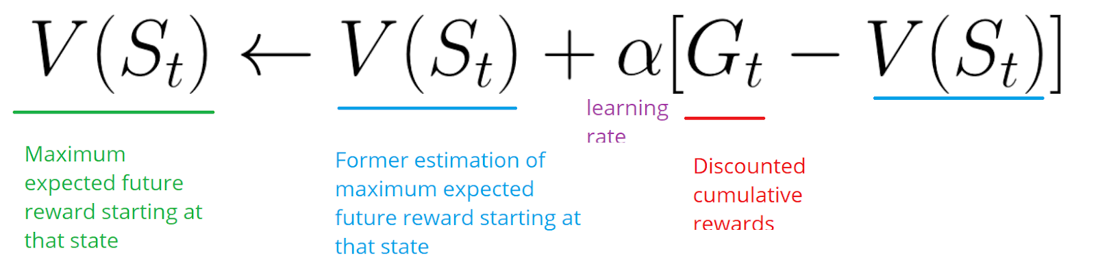
The agent will then update \(V(S_t)\) based on the previous formula.
Then we start a new game with this newly added knowledge.
By running more and more episodes, the agent will learn to play better and better.
Temporal Difference Learning: learning at each time step
TD Learning, on the other hand, does not wait until the end of the episode to update the maximum expected future reward estimation. Instead, TD learning updates its value estimation V for the non-terminal states St occurring at that experience.
This method is called TD(0) or one step TD (update the value function after any individual step).
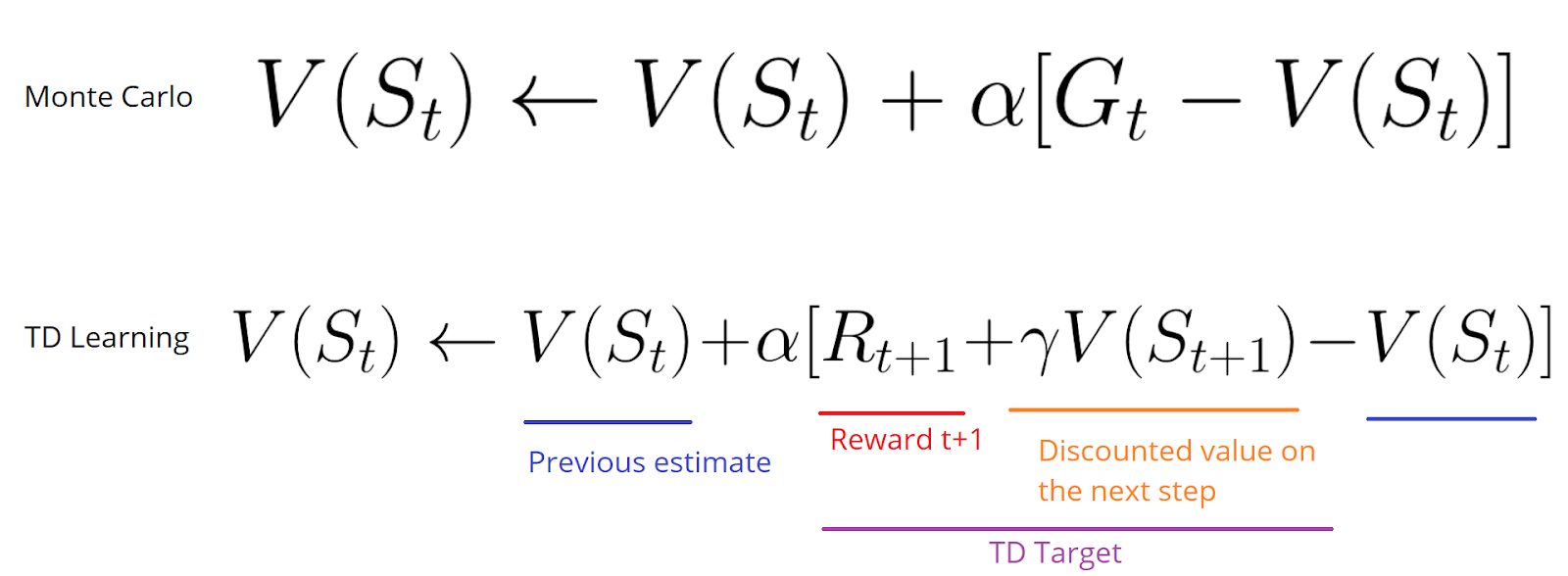
TD methods only wait until the next time step to update the value estimates. At time t+1, they immediately form a TD target using the observed reward \(R_{t+1}\) and the current estimate \(V(S_{t+1})\).
TD target is an estimation; in fact, you update the previous estimate \(V(S_t)\) by updating it towards a one-step target.
Exploration/Exploitation Trade-off
Before looking at the different approaches used to solve reinforcement learning problems, we must cover one more crucial topic: the exploration/exploitation trade-off.
Exploration finds more information about the environment.
Exploitation uses known information to maximize the reward.
Remember, the goal of our RL agent is to maximize the expected cumulative reward. However, we can fall into a common trap.
In this game, our mouse can have an infinite amount of small cheese (+1 each). But at the top of the maze, there is a gigantic sum of cheese (+1000).
If we only focus on the reward, then our agent will never reach the gigantic sum of cheese. Instead, it will only exploit the nearest source of rewards, even if this source is small (exploitation).
However, if our agent does a little bit of exploration, it can find a big reward.
This dilemma is known as the exploration/exploitation trade-off. We must define a rule that helps handle this trade-off.
Three approaches to Reinforcement Learning
Now that we have defined the core concepts of reinforcement learning, let’s move on to the three approaches for solving an RL problem. These approaches are value-based, policy-based, and model-based.
Value-Based
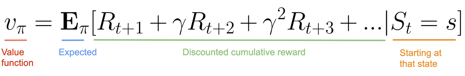
In value-based RL, the goal is to optimize the value function V(s) or an action value function Q(s,a).
The value function tells us the maximum expected future reward that the agent will get at each state.
The value of a given state is the total amount of the reward that an agent can expect to accumulate over the future, starting at the state.
The agent will use this value function to select which state to choose at each step. The agent selects the state with the biggest value.
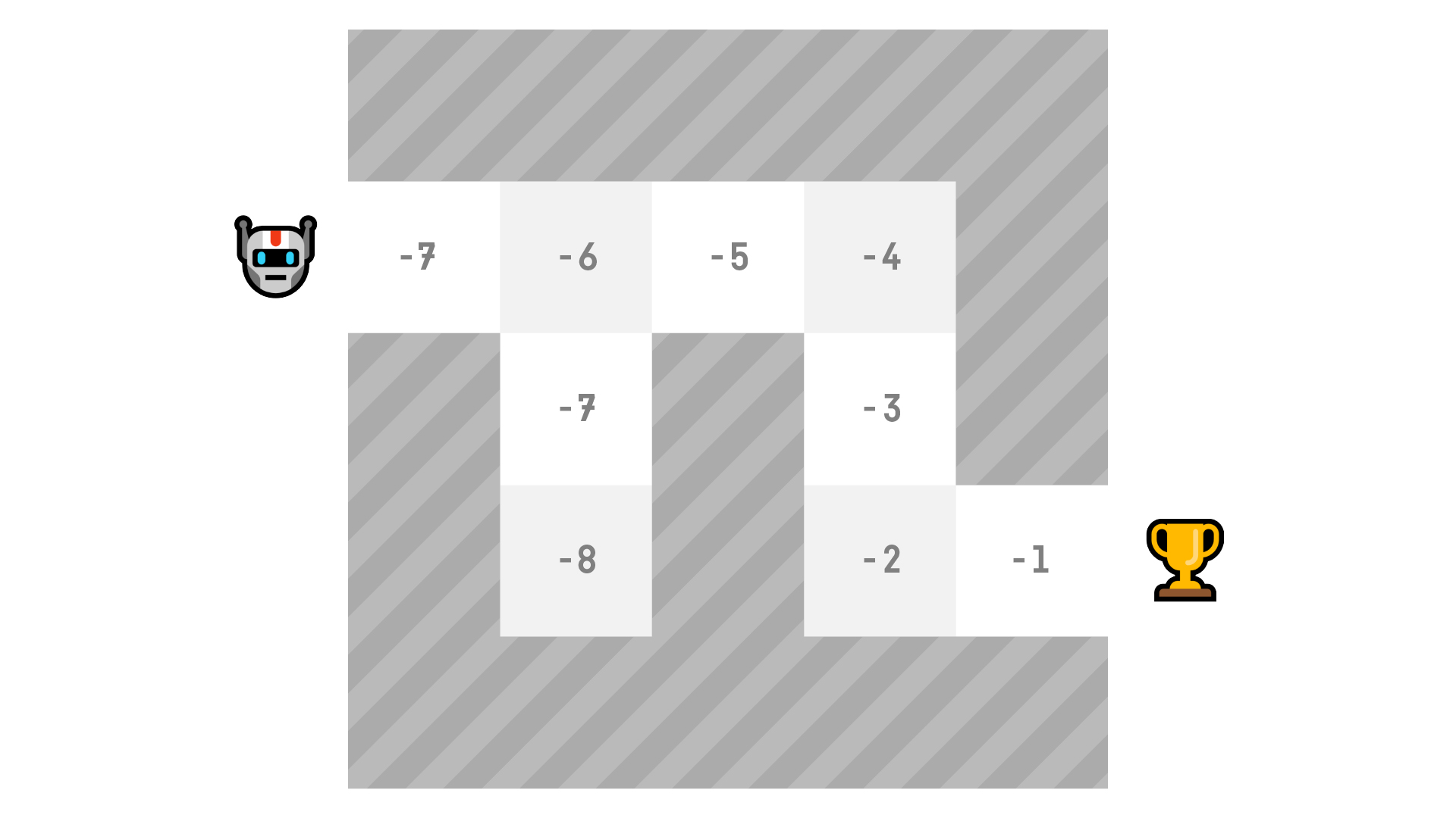
In the maze example, at each step, we will take the biggest value: -7, then -6, then -5 (and so on) to attain the goal.
Policy-Based
In policy-based RL, we want to directly optimize the policy function π(s) without using a value function.
The policy is what defines the agent behavior at a given time.

action = policy(state)
We learn a policy function that lets us map each state to the best corresponding action.
We have two types of policies:
Deterministic: a policy at a given state will always return the same action.
Stochastic: outputs a probability distribution over actions.

Probability of taking that action at that state
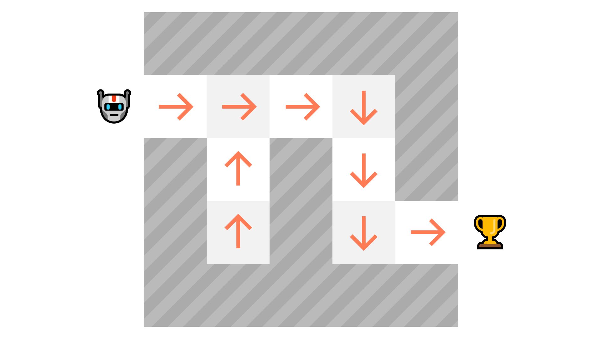
As we can see here, the policy directly indicates the best action to take for each step.
Model-Based
In model-based RL, we model the environment. That is, we create a model that describes the behavior of the environment.
The problem with this approach is that each environment will need a different model representation. Therefore, having a general agent is not the best strategy.
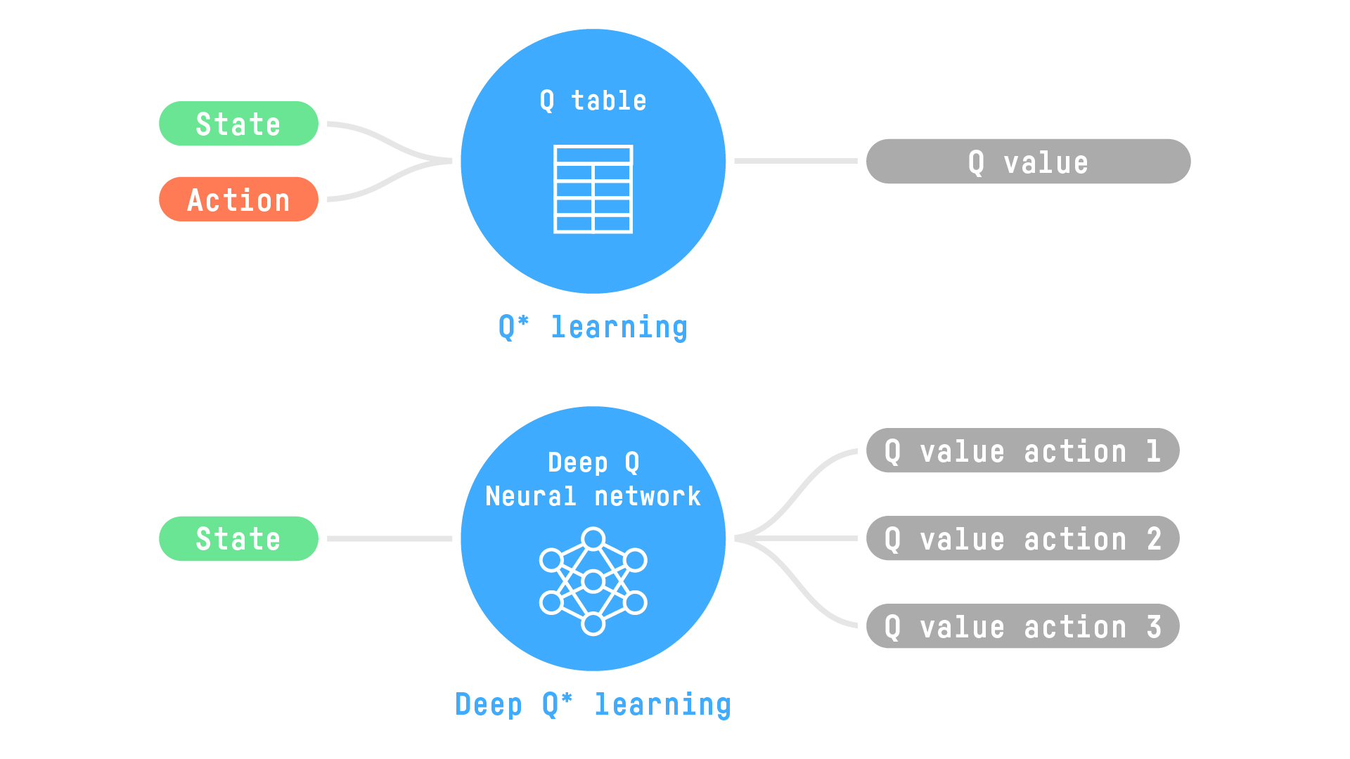
Introducing Deep Reinforcement Learning
Deep reinforcement learning introduces deep neural networks to solve RL problems.
In the upcoming articles, we’ll focus on Q-Learning (classic reinforcement learning) and Deep Q-Learning.
Conclusion
Congrats! There was a lot of information in this article. Be sure to grasp the material before continuing. It’s important to master these concepts before entering the fun part: creating RL agents.
If you want to dive deeper into RL theory, you should read Reinforcement Learning (Sutton & Barto) that is available for free.
Having mastered these RL concepts, you can now choose either the RL Exploration path (to work with the RL plugin within DSS) or the RL in-depth path (to create your agents from scratch, using the notebooks in DSS).
Next, we’ll study our first RL algorithm: Q-Learning. We’ll also implement a Q-Learning agent that learns to play a simple game: Frozen Lake, using the DSS Notebook or the RL plugin, depending on the path that you chose.