How to Leverage Compute Resource Usage Data
This article will guide you through a sample project that will help you keep track of the resource consumption of your DSS flow.
Introduction to Resource Consumption
As a beginner, you can use Dataiku DSS as a standalone application that will handle the data storage, computing, and training of models. However, as your objectives grow, you will want to integrate DSS into a wider ecosystem.
At first, you will typically leverage external data sources (such as remote file storage, relational databases, data warehouses, and so on).
Soon, you will start having more and more computation to do, requesting more power. With the local DSS engine being inherently limited, you will need to leverage external computation technologies. The main and foremost one that Dataiku uses is Spark on Kubernetes, also known as Elastic AI.
Additionally, in order to properly segregate teams and have dedicated UAT or Production servers, you will deploy several DSS instances.
This strategy characterizes the path to success with DSS. However, it comes at a cost. Monitoring the resources used by your DSS instances is a critical topic, especially when the number of projects and users is growing.
Fortunately, Dataiku DSS has an embedded capability to keep track of all those resource requests. This is called Compute Resource Usage (or CRU).
In order to get familiar with this, you will need to read the product documentation on this matter: Compute resource usage reporting
In this article, we will take you through a sample project that will process this raw data into useful metrics and dashboards.
The sample project is provided pre-configured with GCP dataset types but can be changed with other dataset types depending on your platform: MISC-GCP.zip
If you want to use it in another context, you will need to change the dataset types to anything compatible with your platform.
Overview of the Sample Project
This project is designed to be a simple introduction to resource monitoring within DSS. Some specificities are not covered, such as aggregating data from multi-instances. Once you’ve completed this walkthrough, you should have enough knowledge to venture into this yourself.
The first step is to configure the Resource Consumption feature as explained in the documentation.
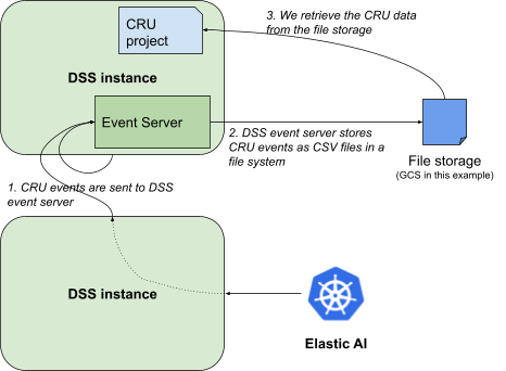
In order to have the correct input, you will need to update the project input dataset, called compute_resource_usage, to match the one you have set up in the Event Server.
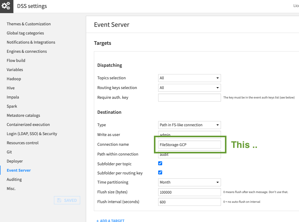
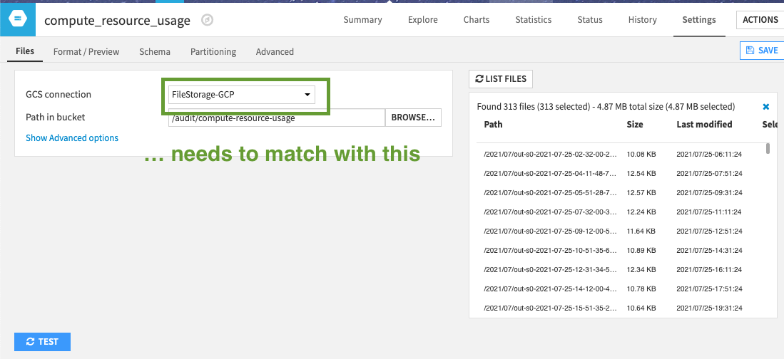
Be careful here also to set the exact path you are using. The DSS Event server can process different types of messages. With the box Subfolder per topic in the Event Server settings, we ensure we find only CRU data in the path /audit/compute-resource_usage.
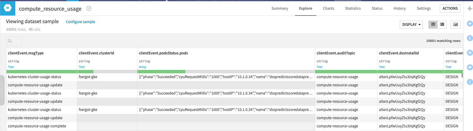
Once all this is done, you can explore the dataset, and you will see the raw data we will use.
Now, you are all set for the ride. First, let’s spend some time explaining what type of information we have in this input dataset.
CRU Explained
If you have read the documentation, you have gone through the “Concepts” paragraph (you should really do it now if you have not: Compute resource usage reporting)
Among other columns, we can highlight some specific entries we will use:
serverTimeStamp - This is the point in time when the resource has been consumed. It will be our X axis on most time-based reports.
clientEvent.msgType - This will help us extract the useful CRU data. If you have Kubernetes activities, you will have entries with kubernetes-cluster-usage-status, which is when DSS stores a status report of the resources consumed by a Kubernetes pod (we look at those in the Kubernetes section).
clientEvent.computeResourceUsage.type - This is the other important triage column as it will tell us which type of resource has been used (LOCAL_PROCESS, SQL_QUERY…).
On top of those, you have many other columns that are specific to each type of CRU report. We’ll review those in each specific section.
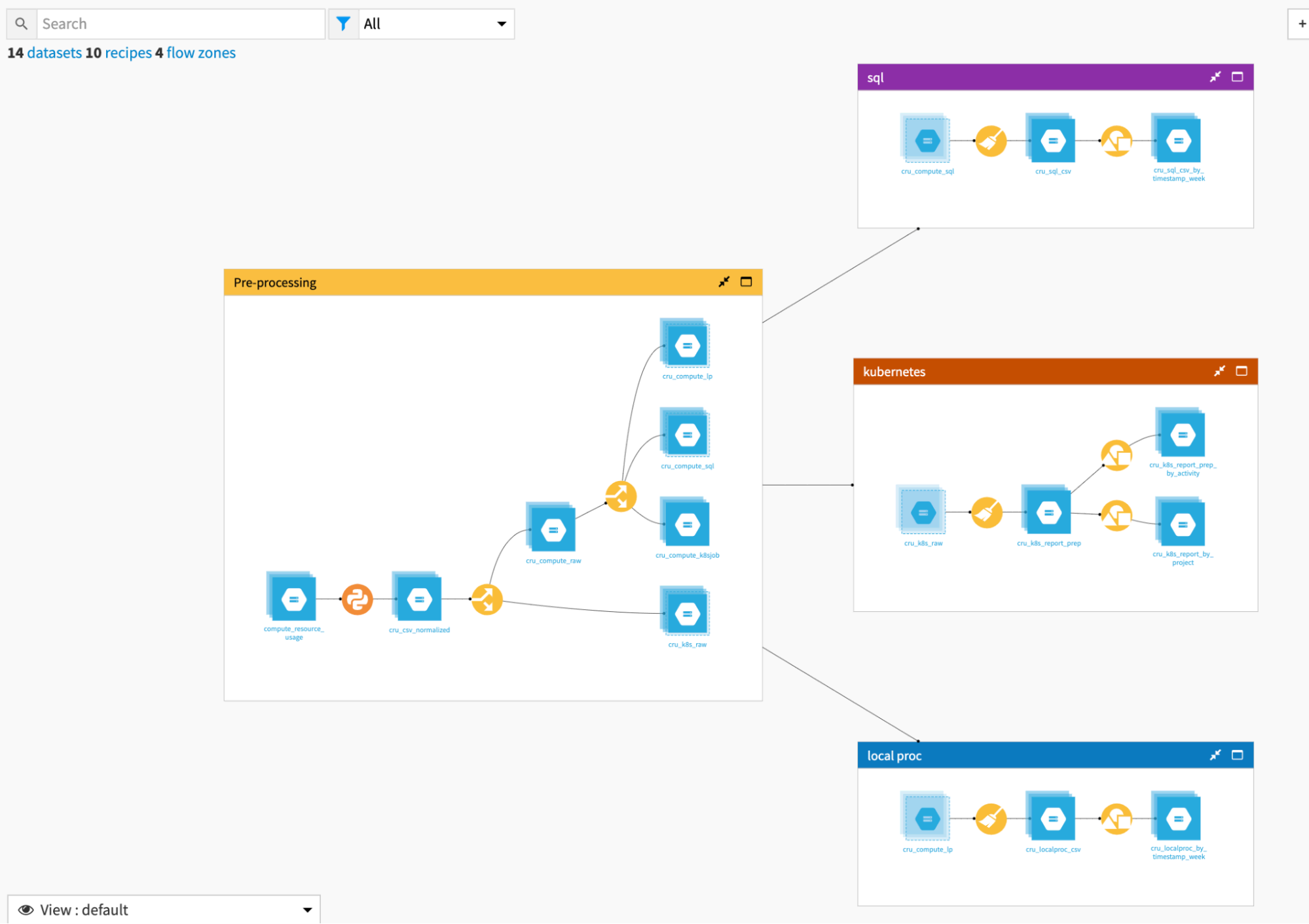
The initial zone, called Pre-processing, mostly deals with splitting the data into the three resource buckets. The other zones are specific to each type of resource.
Kubernetes, as its name states, will leverage mostly the kubernetes-cluster-usage-status from clientEvent.msgType. Those are activity reports fetched directly from the Kubernetes cluster by DSS. This will allow us to analyze the consumption of your Kubernetes cluster(s) across many axes, such as per project, per recipe, per type of activity, etc.
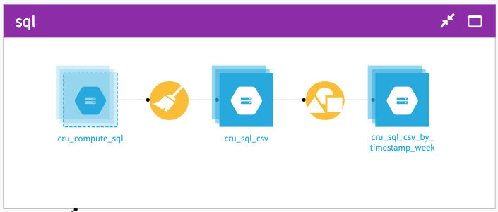
SQL will deal with all SQL requests based on the rows with SQL_CONNECTION & SQL_QUERY from clientEvent.computeResourceUsage.type.
Local Proc will aggregate all data consumed by the DSS engine itself when it works. It is based also on the column clientEvent.computeResourceUsage.type filtered on LOCAL_PROCESS
Let’s deep dive into all of those operations.
Pre-processing
In the Pre-processing zone, the first Python recipe renames and shortens all columns to make data easier to visualize in Dataiku DSS. It’s not mandatory or very complex, but a practical step.
For example, the column clientEvent.computeResourceUsage.localProcess.cpuUserTimeMS will be renamed as evt_cru_loc_cpuUserTimeMS.
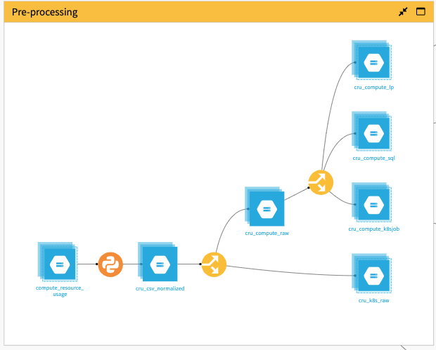
The next recipe is a Split recipe that pushes Kubernetes reports on a specific path (cru_k8s_raw) using the column evt_msgType.
The second Split recipe splits the other rows according to evt_cru_type, and pushes them into three different datasets:
one for all SQL processing (cru_compute_sql),
one for local processor (cru_compute_lp), and
one for the local Kubernetes processing (cru_compute_k8sjob)
In the end, there is nothing very complex here–mostly data splitting.
One thing to note is that some rows from the original CRU data are dropped and never used. This is normal and concerns the start and finishing Kubernetes task reports that are of no use.
Kubernetes
The Kubernetes zone processes the Kubernetes data into usable CPU and RAM usage numbers.
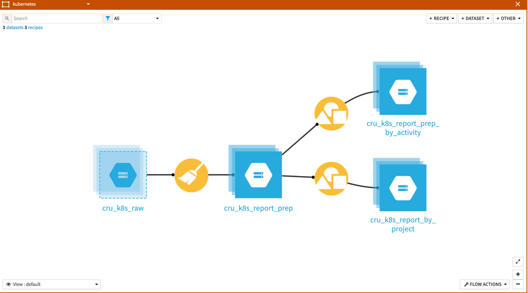
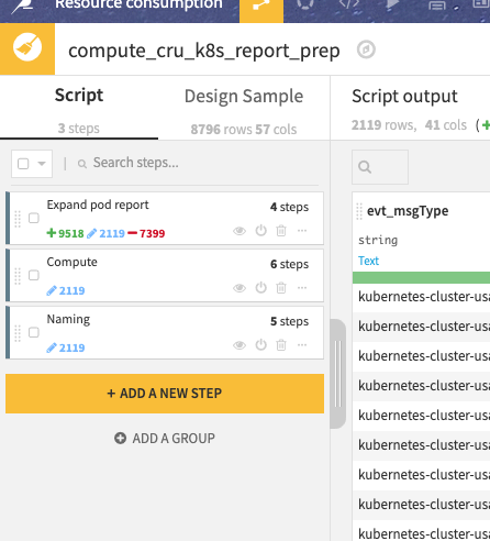
Most of the work is done in the Prepare recipe, which is organized into three groups of operations:
Expand pod report - The initial step is to expand the pod reports, which are stored in JSON format originally in the clientEvent.podsStatus.pods column. The important point to note is that we will keep only the report with phase=”Running”. You may have a lot of lines with other statuses, but they do not hold meaningful information regarding the k8s usage.
Compute - We create a set of computed fields for the CPU and RAM consumption. There are various flavors that we compute: one is the basic usage, another is the unit of consumption per hour, and the last is the related cost (using a simple formula).
Naming - This is more for cosmetic usage where we clean, rename, and reorganize the columns.
In these steps, the main one is clearly the second so let’s take some time to go a bit deeper in computation with one example: computing k8s_cpu_millis.
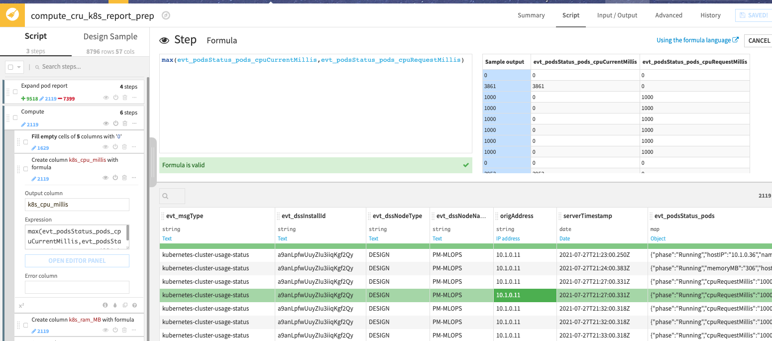
The JSON report we have from Kubernetes contains two CPU information: evt_podsStatus_pods_cpuCurrentMillis and evt_podsStatus_pods_cpuRequestMillis.
Those two pieces of information are originally coming from the kubectl command: kubectl top pod for cpuCurrentMillis and kubectl get pods for cpuRequestMillis.
cpuRequestMillis is what we CPU DSS has requested, the minimal reserved CPU consumption
cpuCurrentMillis is the actual CPU consumption
If the current CPU consumption is below the requested one, we need to count the requested value, because that is what DSS asked Kubernetes to reserve, even if it consumes less.
If the current CPU consumption is above the requested, we take its value, as this means the job is consuming that amount of CPU.
To do that simply, we build a formula that takes the maximum of the two metrics.
If you are further interested in Kubernetes metrics and their usage, we can recommend the great blog entry from Datadog Collecting Metrics With Built-in Kubernetes Monitoring Tools.
The other formulas in this group are very similar, dealing with RAM or with other time ranges for usage, as we need the consumption in CPU/hour for cost.
In the end, in this sample, we use a simple formula to compute the cost, which takes a flat cost for RAM (0.004237$ for each 1 hour of 1Gb) and CPU (0.031611$ for each 1 hour of 1 CPU). Those numbers are sample costs taken from Google GCP on-demand pricing for n1 machines us-central1 at the time of the writing of this article.
You obviously need to revisit this cost as it may depend on many other elements. The last two grouping recipes are to facilitate the building of dashboards.
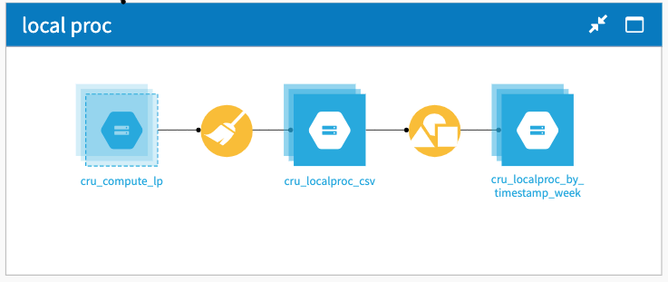
Local proc
The Local proc zone primarily contains a Prepare recipe with all of the needed transformations. The Group recipe is used to have some data correctly computed for our dashboards.
Let’s look at the Prepare recipe:
The first processor just helps us have fewer columns, a cosmetic step.
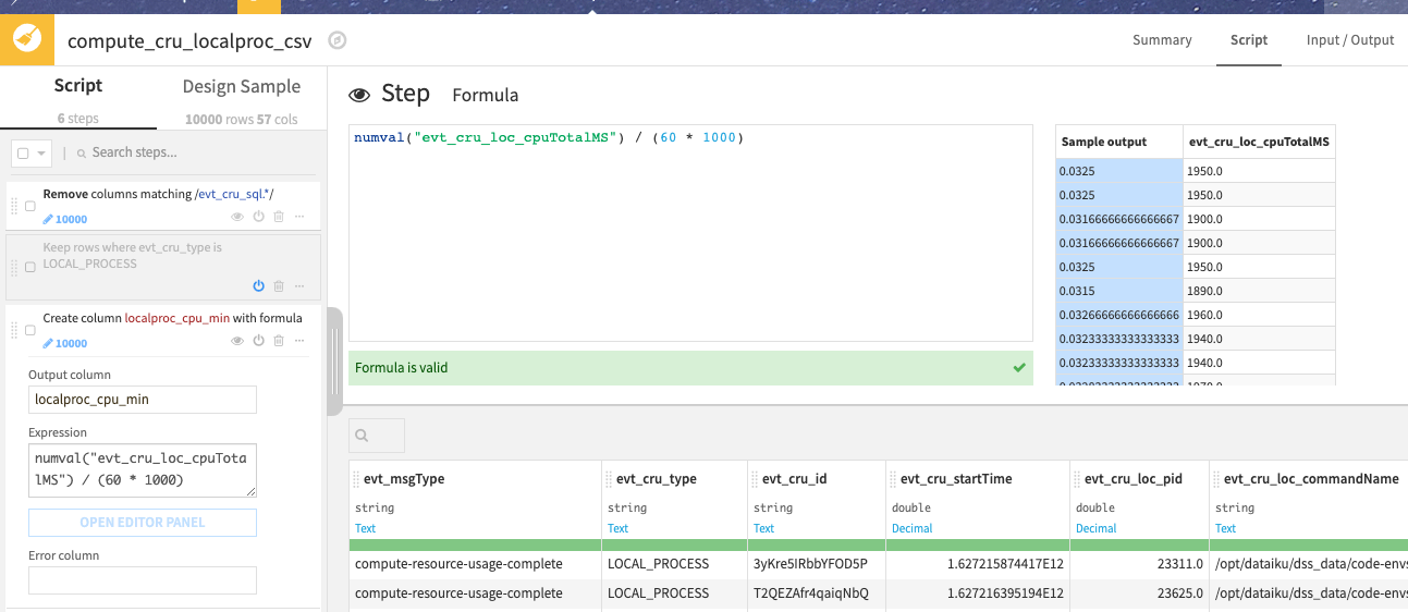
The others are where we compute actual usage. You can look at them but there is very little complexity as the CRU data is already good to use. Most of the work is to group the consumption of CPU and RAM in specific time intervals, as milliseconds is not very practical.
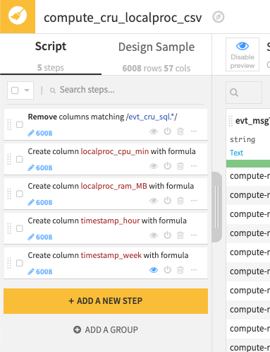
The last grouping is used for specific metrics computations for the dashboards.
SQL
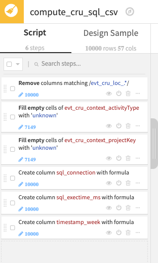
The SQL zone is very similar to the Local proc zone, as it also mostly relies on some cleanup and computation done in the Prepare recipe.
In the Prepare recipe:
The first processor is for cleanup and readingness.
The following two are to fill current gaps we have in the action reporting with explicit values to be clearer.
The next aggregate the name of the connection in a single field (as it is different between SQL_CONNECTION & SQL_QUERY).
Next, we compute the actual metric we want to follow, which is the execution time of each SQL request, using different time intervals.
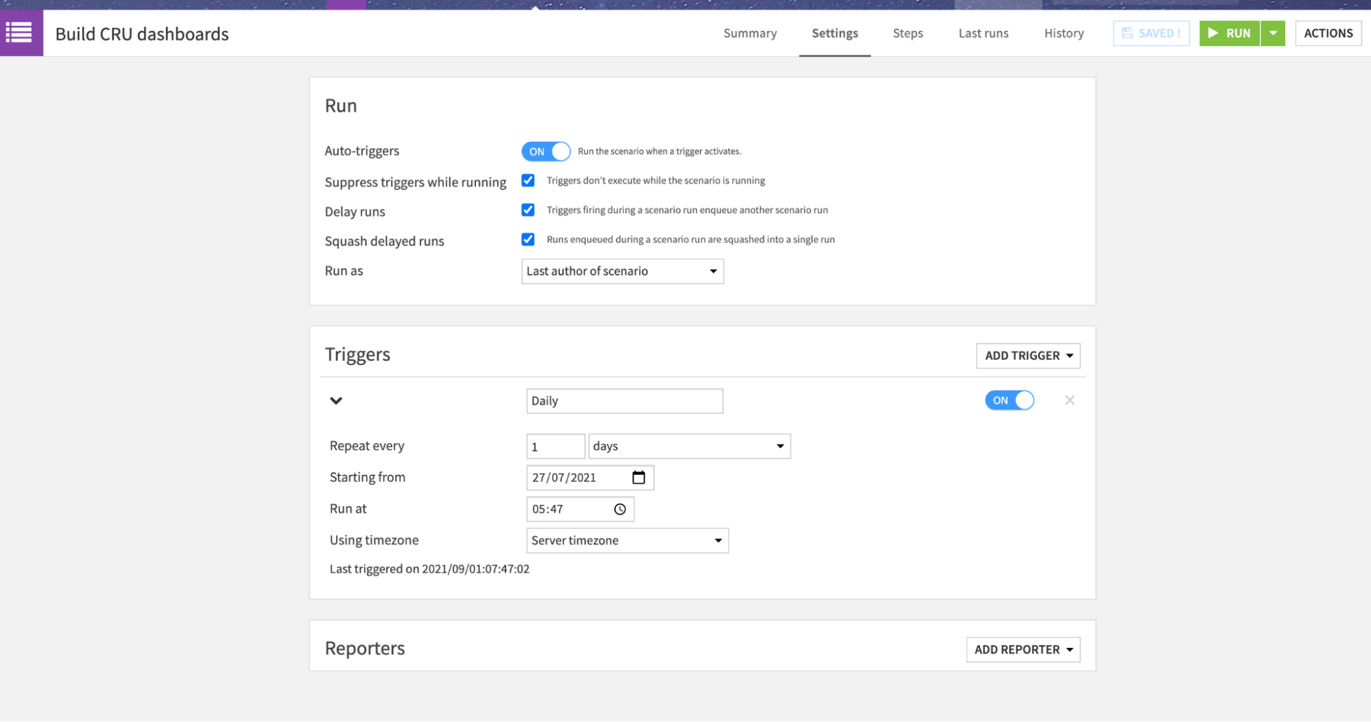
Running the Flow
Now that we have reviewed in detail all the zones and what they do, it is time to build it.
The project contains a pre-packaged scenario that builds the output datasets. You can execute it. Once validated, you can make it trigger automatically every day, and let it run for a few days or weeks in order to have a starting picture of your consumption.
Further Work
You can find below some notes on specific behaviour or voluntarily ignored subtlety that you may want to investigate, and add to this flow:
Regarding Kubernetes data when using Spark, there are also resources consumed on the local DSS server. Should you want to add those into the final data, you need to join the cru_k8s_report_prep and the cru_compute_k8sjob datasets using the executionId column.
If you are building this report with multiple instances of DSS, you will need to use the clientEvent.dssInstallId from the input dataset, this will tell you which one has consumed resources (You also have clientEvent.dssNodeName, which has a more meaningful value, but is not mandatory and can change).
If you are using multiple instances of DSS with Elastic AI leveraging the same Kubernetes cluster, you will end up with duplicate lines. This is due to the fact that each instance will report the Kubernetes cluster raw report. In order to avoid that, you need to enable the Kubernetes resource usage reporting on only one instance (This is in Administration > Settings > Misc.). Alternatively, you can filter out the CRU data in the Flow, but that is less efficient.
Reports
The project is delivered with sample dashboards. They should work out-of-the-box once you start having actual data. Here is a sample export: FinOps-dashboard.pdf
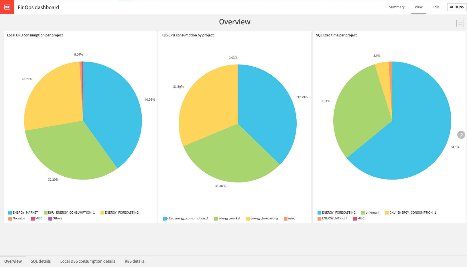
The dashboard has four tabs:
Overview - This tab takes a single metric from the three sub-flows as an overview and splits the usage by project.
SQL Details - This tab has one time-based graphic on the SQL execution time and splits consumption three ways - one per usage type, one per connection, and another per project.
Local DSS consumption details - This one focuses on the local DSS server, and is organized similarly with consumption split four ways - per context and per project, each for CPU and RAM.
K8S details - This is a more specific dashboard that takes a time-base evolution as others, but then identifies the most CPU and RAM intensive projects and activities.
Of course, this dashboard is just an example, and many more graphics or metrics can be built. Reviewing and changing those dashboards is probably the first and foremost task you have to work on as you need to make them fit your needs. In a FinOps approach, the ideal scenario is to discuss with other stakeholders (business, projects, IT, finance…) to review which information they need, and progressively enrich the dashboards.