Hands-On Tutorial: Forecasting Time Series (Visual ML Interface)
Today many machine learning problems often involve a time component. This additional temporal constraint introduces complexities that require careful analysis.
Dataiku offers various ways to implement time series modeling and forecasting. We’ll focus on Dataiku’s time series analysis functionality in the visual machine learning interface. You’ll get to see how this interface offers users the same capabilities for time series forecasting as for any other type of Machine learning model.
Let’s Get Started
In this tutorial, you’ll use the visual time series functionality of the Lab to design and train a model on time series in a dataset. You’ll then deploy the model to the Flow, evaluate the model, and, finally, score it. You’ll perform these tasks by using visual interfaces within the visual machine learning framework.
Prerequisites
A Dataiku 11 instance
A basic level of knowledge about Dataiku is helpful. If you’ve never used Dataiku before, try the Core Designer learning path or a Quick Start tutorial.
A code environment that includes the required packages for time series forecasting models. You can create a new code environment that includes these packages or add them to your existing code environment. See the Requirements for the code environment in the product documentation.
Tip
To implement time series analysis, you’ll need to specify this code environment in the visual ML interface.
Create the Project
From the Dataiku homepage, click +New Project > DSS Tutorials > Time Series > Forecasting Time Series With Visual ML (Tutorial).
Note
You can also download the starter project from this website and import it as a zip file.
Build the Flow
The initial starter Flow contains empty datasets. To work with these datasets, we’ll need to build the Flow.
Click Flow Actions from the bottom-right corner of your window.
Select Build all and keep the default selection for handling dependencies.
Click Build.
Wait for the build to finish, and then refresh the page to see the built Flow.
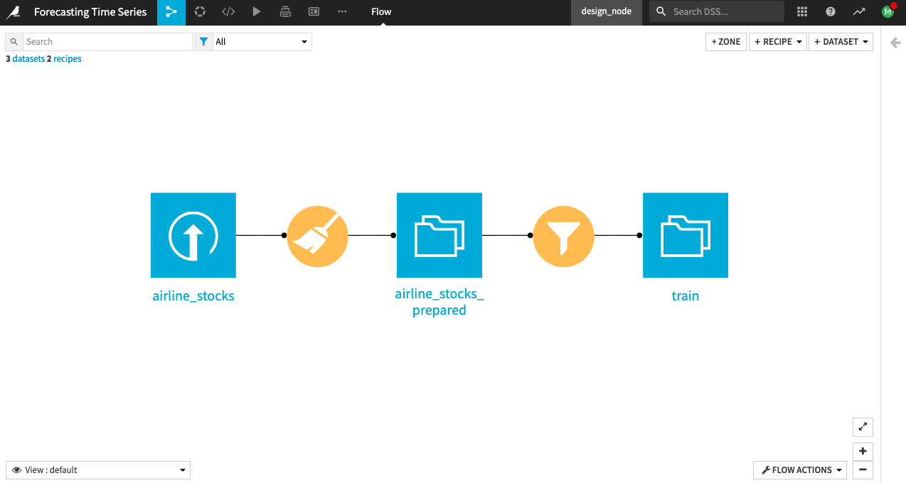
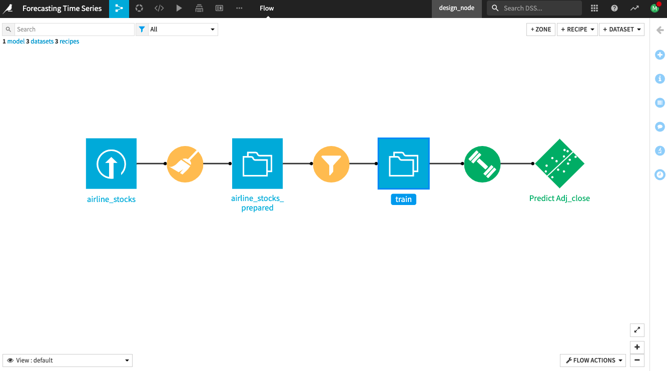
Description of the Starting Flow
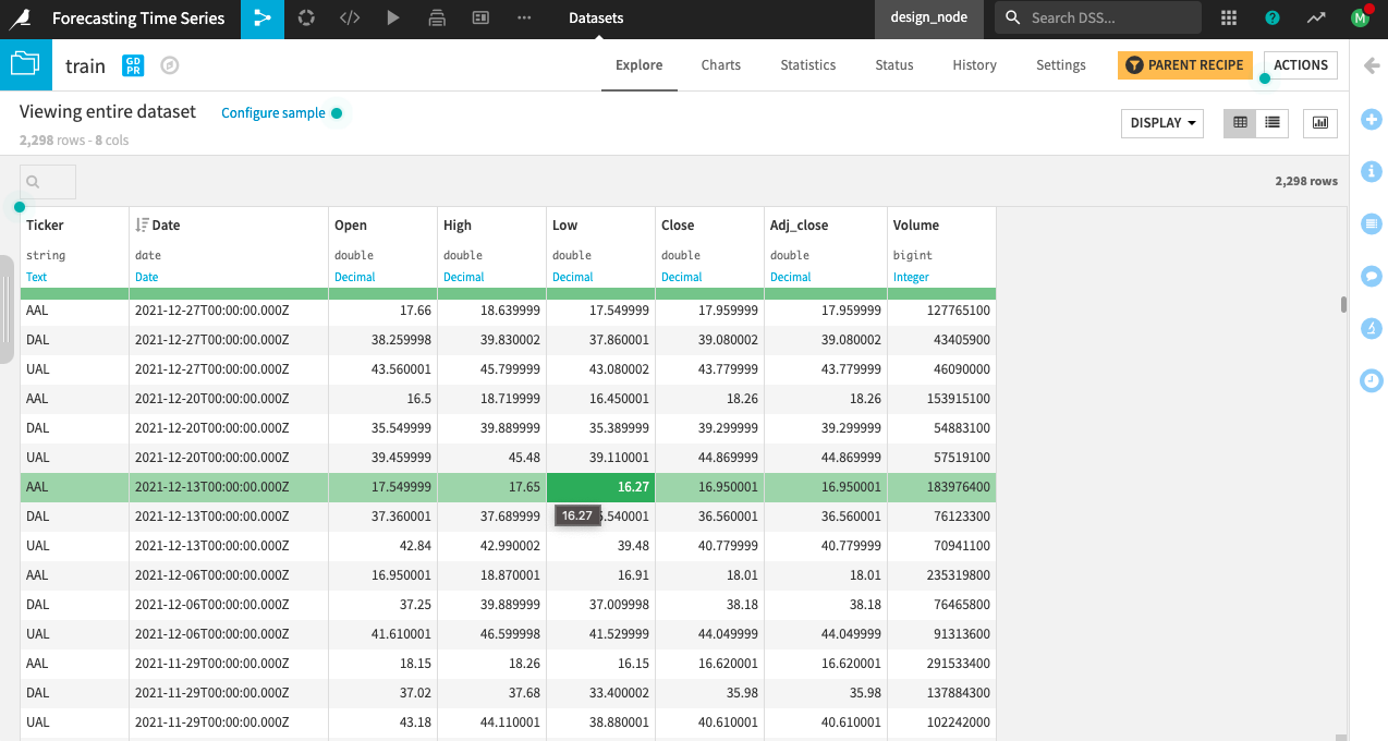
The project begins with an input dataset, airline_stocks, that contains weekly stock prices from 2008 to January 2022 for three major US airlines: American (AAL), Delta (DAL), and United (UAL). The dataset contains the following columns:
Ticker: Stock symbol used to identify each time series in the dataset uniquely
Date: weekly time stamps
Open, High, Low, Close: corresponding opening, highest, lowest, and closing prices for the day
Adj Close: the adjusted closing price for the day
Volume: the number of stocks traded
A Prepare recipe applied to the input dataset (airline_stocks) parses the Date column and renames the Adj Close column to Adj_close. Adj_close is the target variable that you’ll forecast. This data preparation in the Prepare recipe is all you need for the input dataset, as it is generally clean with no missing values.
The project also includes a training dataset train filtered out of the prepared airline_stocks_prepared dataset. The train dataset contains stock data for the Monday of every week from 2008 to the end of December 2021.
Note
The airline_stocks_prepared dataset contains all the training and validation data and will be useful during model evaluation and scoring. This is because Dataiku requires that the input datasets to the Evaluate and Scoring recipes include the historical (training) data used by the time series model.
First, view the Charts tab of the train dataset to see some pre-computed plots of the Adj_close price in train. The Statistics tab of the dataset also includes some pre-computed analyses on the Adj_close price of the UAL time series in train.
Plotting your data and performing statistical analyses are good initial steps to see if you can observe any patterns in the time series, such as trends and seasonalities.
Tip
To explore the dataset using charts and statistical analyses, see the “How-To: Perform Statistical Analysis on Time Series” article.
Build and Train a Time Series Model
To build the time series model, you’ll use the train dataset. This dataset contains all the time series data before January 1, 2022.
Tip
You’ll use the remaining time series values (occurring after January 1, 2022) as a validation set to evaluate the performance of your trained model. This validation set contains 18 weekly entries (or time steps) for each stock price time series.
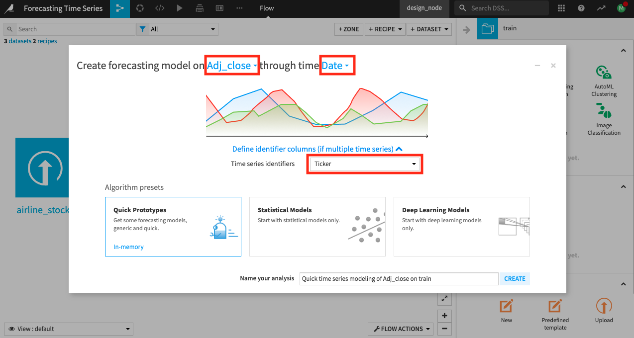
Create the Time Series Forecasting Analysis
To create the time series forecasting analysis:
Click the train dataset in the Flow.
Select Time Series Forecasting in the Lab section of the right panel.
Specify Adj_close as the numerical feature and Date as the date feature.
Select Ticker as the identifier column for multiple time series (remember, we have time series for three different airlines).
Select Quick prototypes and create the analysis.
Now you can examine the Design tab of the analysis.
Inspect the General Settings Panel
In the General settings panel of the Design tab, Dataiku already specified parameter values based on the input selections you made when you created the forecasting analysis and based on default settings. Examine these values.
For the Time step parameters, Dataiku already specified the time step as “1 week”.
Change the “Day of week” to Monday, as the weekly values in the dataset all occur on Mondays.
Note
Although the input data here is equispaced, it is important that you specify the correct value for the Day of week parameter. Suppose you select a weekday different from the day the timestamps occur. In that case, Dataiku will create new timestamps for the specified day of the week and determine their corresponding values (for other columns in the dataset) by interpolating between the original timestamp values.
The Scoring and Evaluate recipes will also forecast values for dates that fall on the weekday you specify.
Also, notice the Forecasting parameters.
Specify the “Forecast horizon” as
6. This parameter determines the length of the model forecast; therefore, you should specify a value that is a factor of the length of the validation set.
Note
Recall that the validation set contains the time series values occurring after January 1, 2022. This data is in the airline_stocks_prepared dataset and contains 18 weekly entries (or time steps) for each stock price time series.
Dataiku allows you to re-detect settings when you change the forecasting horizon.
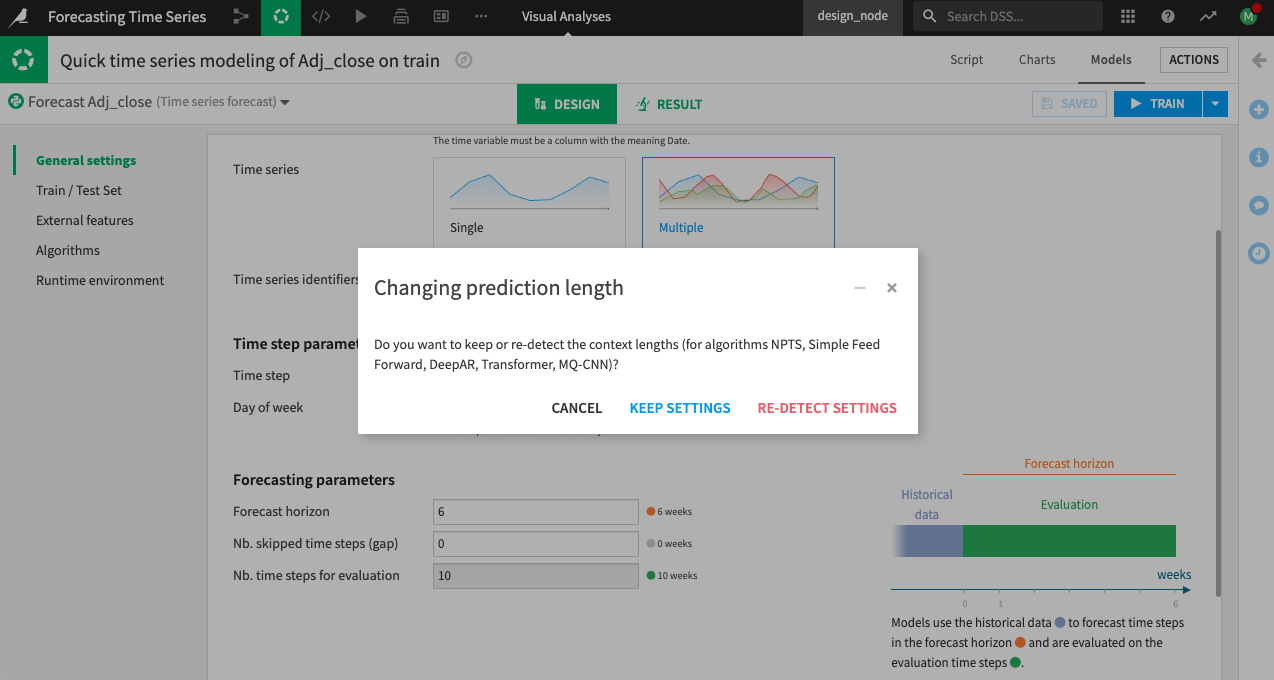
Click Re-Detect Settings.
Dataiku changes the “Nb. time steps for evaluation” to 6 after re-detecting settings.
Tip
Notice the graphic to the right side of the “Forecasting parameters”. Visual aids like this appear throughout the visual time series interface to help you understand how Dataiku uses the parameter values you specify.
Also, notice the forecasting quantiles. Keep these default values.
Note
Note that Dataiku will use the same Forecast horizon value when you apply a Scoring recipe to the model. Dataiku will also use the Nb. Time steps for evaluation value as the forecast horizon when you apply an Evaluate recipe to the model. Finally, Dataiku will use the same Forecast quantiles you specify during training when you score and evaluate the model.
Go to the Train/Test Set panel to examine it.
Inspect the Train/Test Set Panel
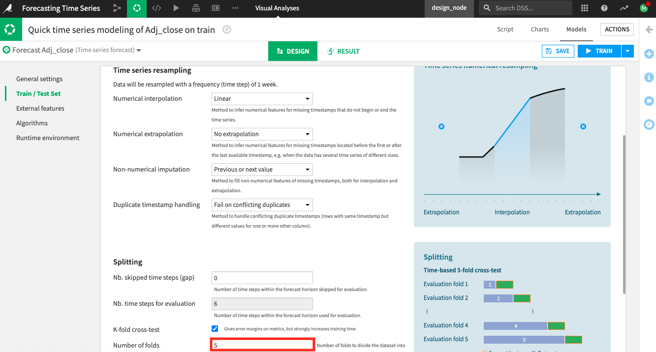
In the Train/Test Set panel, you can specify settings for resampling and splitting the time series.
Note
If the train data is not equispaced, Dataiku will automatically resample it. You’ll also be able to specify the imputation method for numerical and categorical data in the missing time steps.
Keep the default “Time series resampling” settings.
Select the K-fold cross-test splitting strategy checkbox in the section for the Splitting parameters.
Keep the default
5folds to use for the k-fold cross-test.
Note
Using the cross-test provides a more accurate estimation of model performance and is useful when you don’t have much training data. The product documentation on Settings: Train/Test set explains how the process works.
Go to the External Features panel.
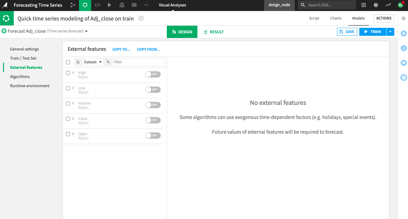
Inspect the External Features Panel
External features are exogenous time-dependent features. By default, Dataiku disables the external features for several reasons. One reason is that some training algorithms do not support the use of external features.
Another reason for this default behavior is that for any model you train with external features, Dataiku will require you to provide future values of those external features during forecasting (when trying to score the trained model). Therefore, if there’s no way to know the values of the external features ahead of time (as it applies in this case of stock price information), the model should not use them during training. Using these features will lead to what is called “data leakage”.
Leave the external features disabled.
Go to the Algorithms panel.
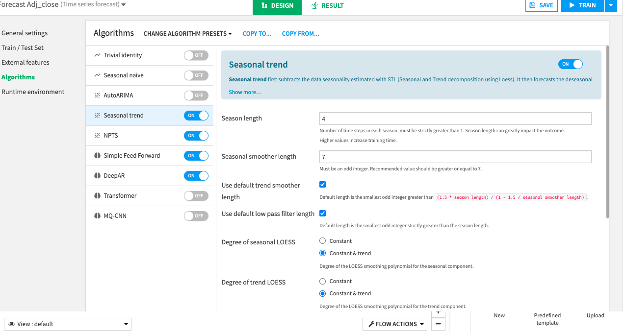
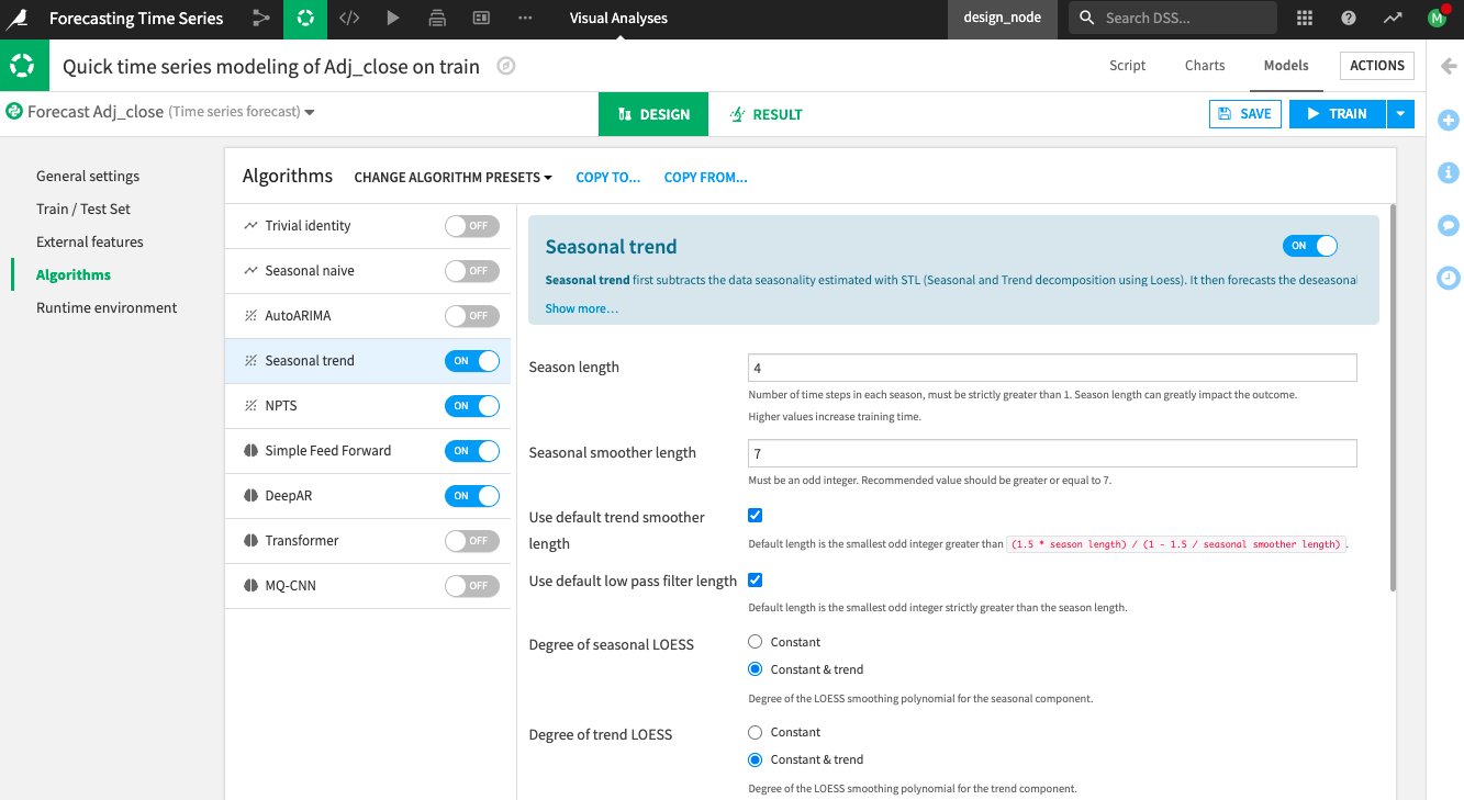
Inspect the Algorithms Panel
Dataiku provides several algorithms that you can use to train your model. By default, Dataiku selects the NPTS and Simple Feed Forward algorithms.
Enable the Deep AR and Seasonal Trend algorithms in addition to the default selections.
One last step before training is to check the runtime environment.
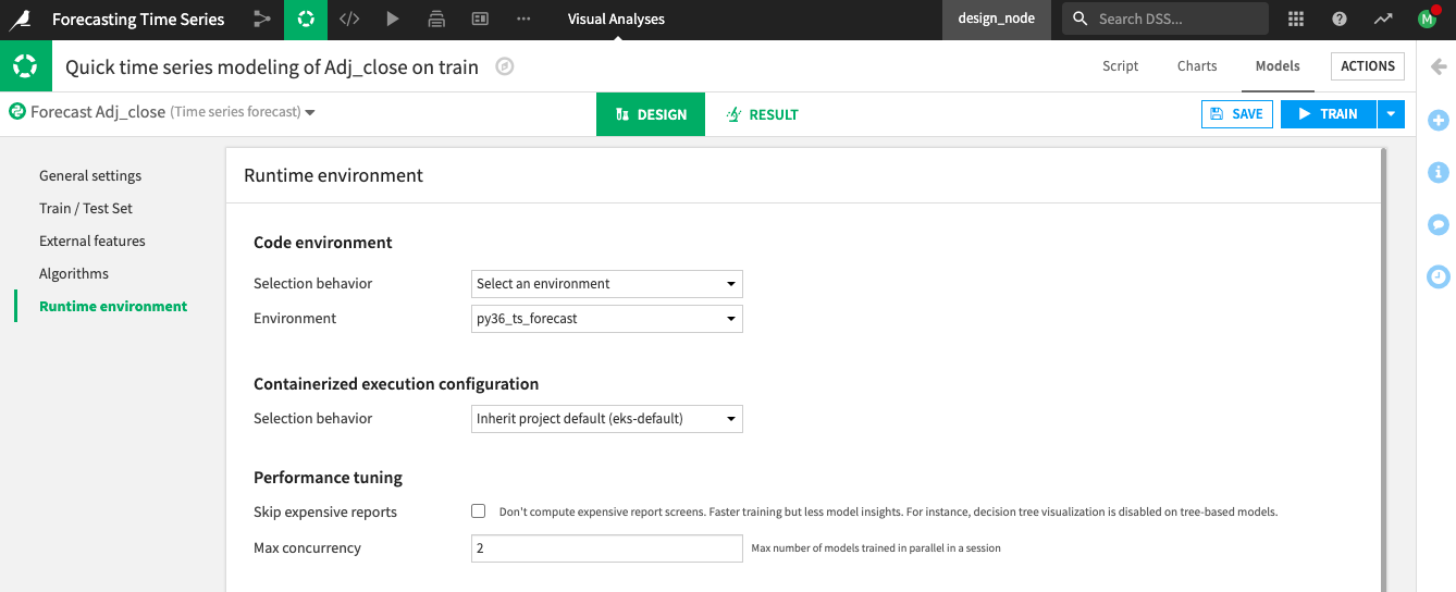
Inspect the Runtime Environment Panel
From the Runtime environment panel, you can select the code environment that contains the required packages for building the time series forecast models.
Go to the Runtime environment panel.
Select a code environment that includes the required packages for time series forecasting models.
Note
You can create a new code environment that includes the required packages or add them to an existing code environment. See the Requirements for the code environment in the product documentation.
Click Train, and then Train once more to begin training the models.
Inspect the Training Results and Deploy the Model to the Flow
You can inspect the results for the models you trained, just as you would for prediction or clustering models.
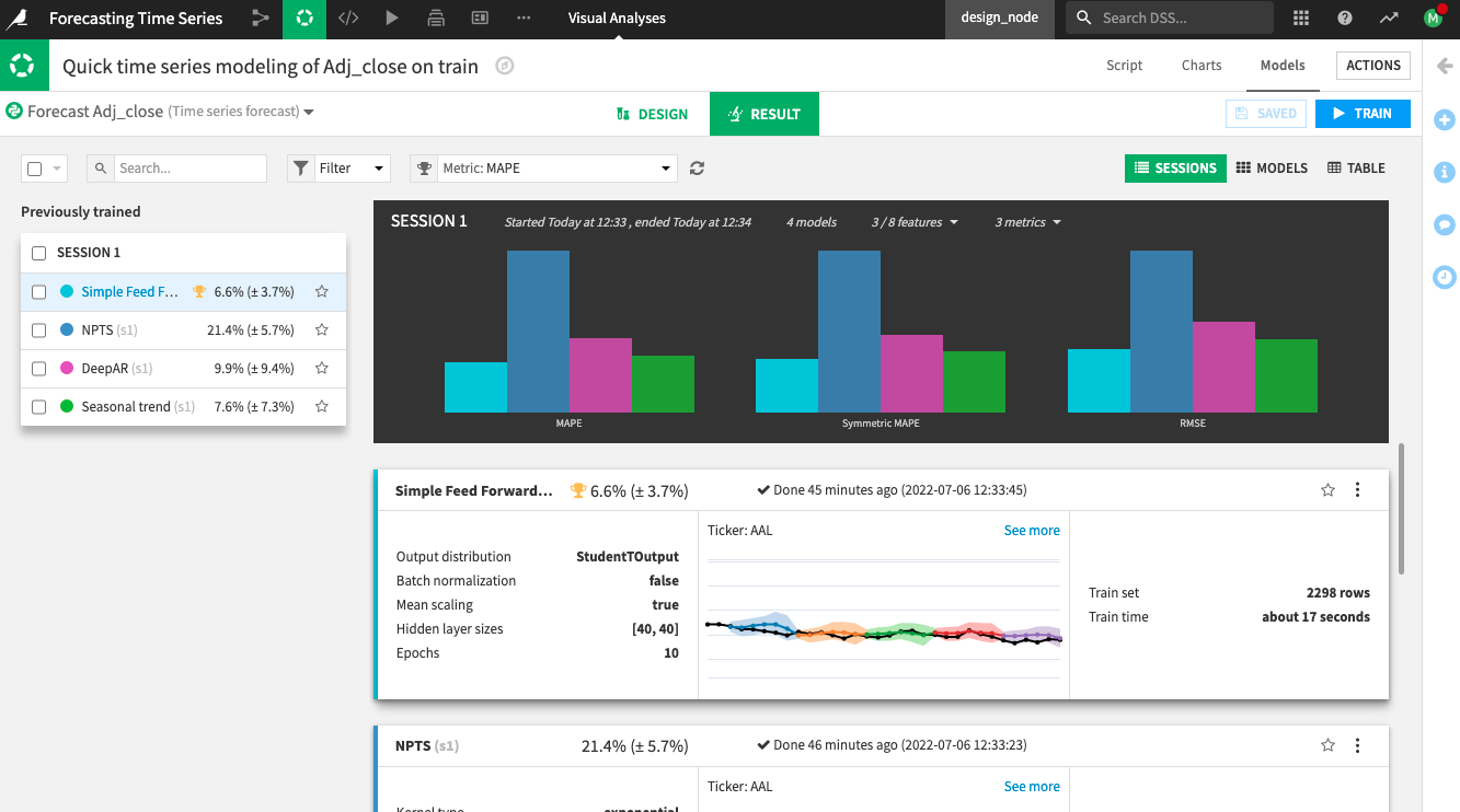
Notice the bar charts at the top that allow you to compare different metrics across the trained models. The Simple Feed Forward algorithm performed best for all three metrics (MAPE, Symmetric MAPE, and RMSE).
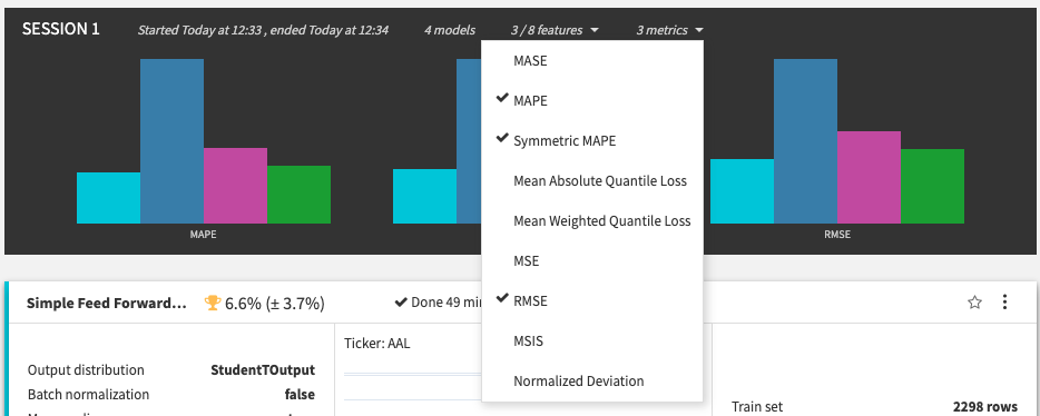
You can click the metrics dropdown in the session summary to change the displayed metrics and see more performance information across the algorithms.
On the Model Result page, click the best-performing model, Simple Feed Forward, to see the model training results.
Click the Forecast values panel to see the predictions for each time series (AAL, DAL, and UAL) and inspect the plots.
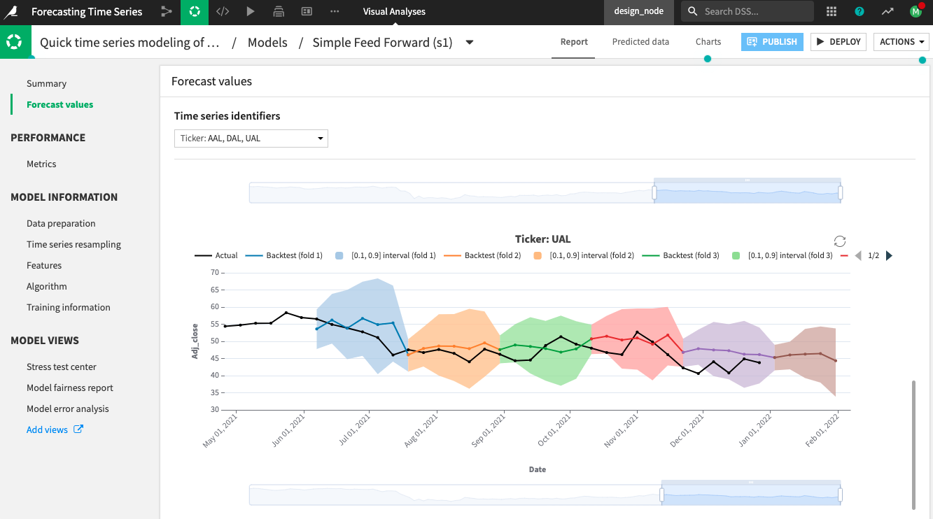
For each of the “k = 5” folds, a black line shows the actual time series values; another line shows the values that the model forecast for that fold; and a shaded area represents the confidence intervals for the forecast values.
Notice that Dataiku also plots the forecast values and confidence intervals for the next horizon of the training dataset (beyond the last timestamp in the training data).
The other panels of the model’s Report page show additional training details. For example, the Metrics tab in the Performance section displays the aggregated metrics for the overall dataset and its individual time series. The tabs in the Model Information section provide more details on resampling, features used to train the model, the algorithm details, etc.
Once you finish inspecting the model and are satisfied with its performance, you can deploy the model to the Flow, as you would for any prediction model in Dataiku.
Click Deploy from the top right corner of the page.
Click Create to deploy the Predict Adj_close model to the Flow.
Note
Like any other Dataiku visual ML model, you can deploy time series models in the Flow for batch scoring or as an API for live scoring.
Evaluate the Time Series Model
Next, evaluate the model’s performance on data not used during training. For this, you’ll use the Evaluate recipe.
Create the Evaluate Recipe
To apply the Evaluate recipe to the time series model, you’ll use a validation set from the airlines_stocks_prepared dataset as input. The validation set will include the time series values after January 1, 2022. Recall that this validation set contains 18 weekly entries (or time steps) for each stock price time series.
To create the Evaluate recipe,
Click the model to select it from the Flow.
Click the Evaluate recipe from the right panel.
Specify airline_stocks_prepared as the “Input dataset” to the Evaluate recipe.
Click Set to add an “Output dataset”.
Name the dataset
eval.Click Create the Dataset.
Click Set to add a “Metrics” dataset.
Name the dataset
metrics.Click Create the Dataset.
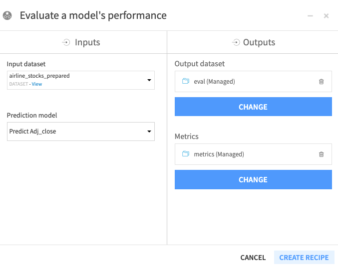
Click Create Recipe.
Dataiku opens up the recipe’s Settings page.
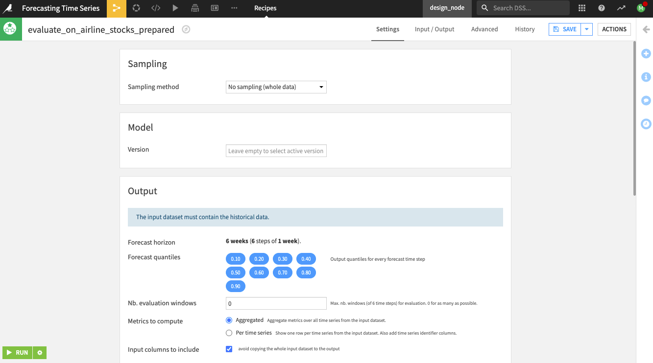
Notice the following on the Settings page:
Dataiku alerts you, “The input dataset must contain the historical data.”
Note
If you used external features while training the model, Dataiku would require that the input data to the Evaluate recipe contain values for the external features. This requirement is also true when you use the Scoring recipe.
By default, the recipe uses a forecast horizon of six weeks (six steps in advance) since this was the model’s setting during training. Dataiku also outputs forecast values at different quantiles (the same ones used during training).
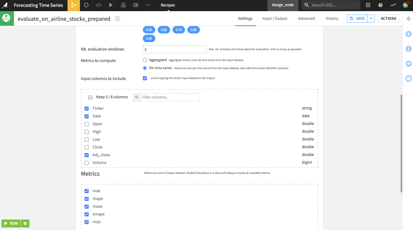
Specify the remaining settings for the recipe as follows:
Specify the “Nb. evaluation windows” values as
3to use three evaluation windows of 6 weeks.
Tip
Notice that we chose these settings strategically to ensure that the Evaluate recipe forecasts the time series values for all the 18 time series values not used during training.
Select the option to compute metrics “per time series” for Dataiku to show one row of metrics per time series (note that you can also compute aggregated metrics).
Keep the default selection of the columns to include in the output dataset eval and the metrics dataset metrics.
Run the recipe.
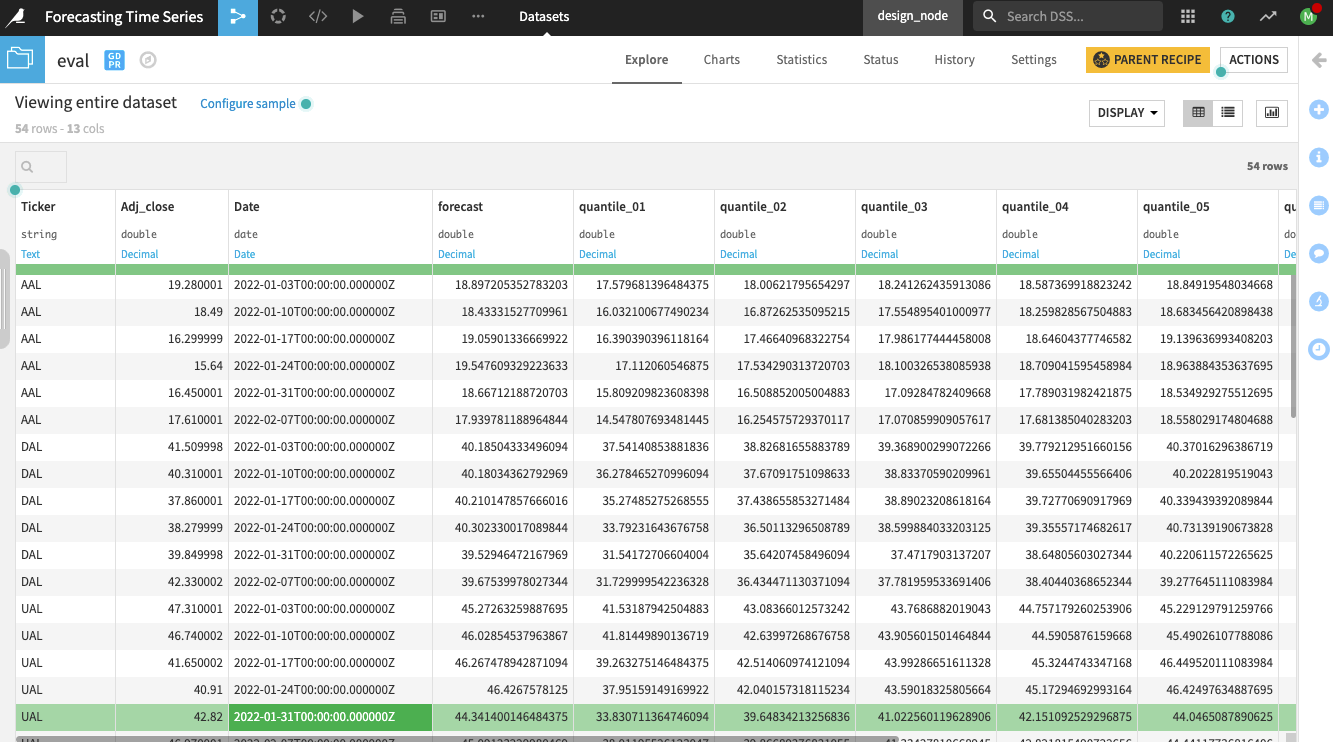
Explore the Evaluation Results
In the eval dataset, you can view the actual values of the Adj_close prices and the forecasts alongside the quantiles.
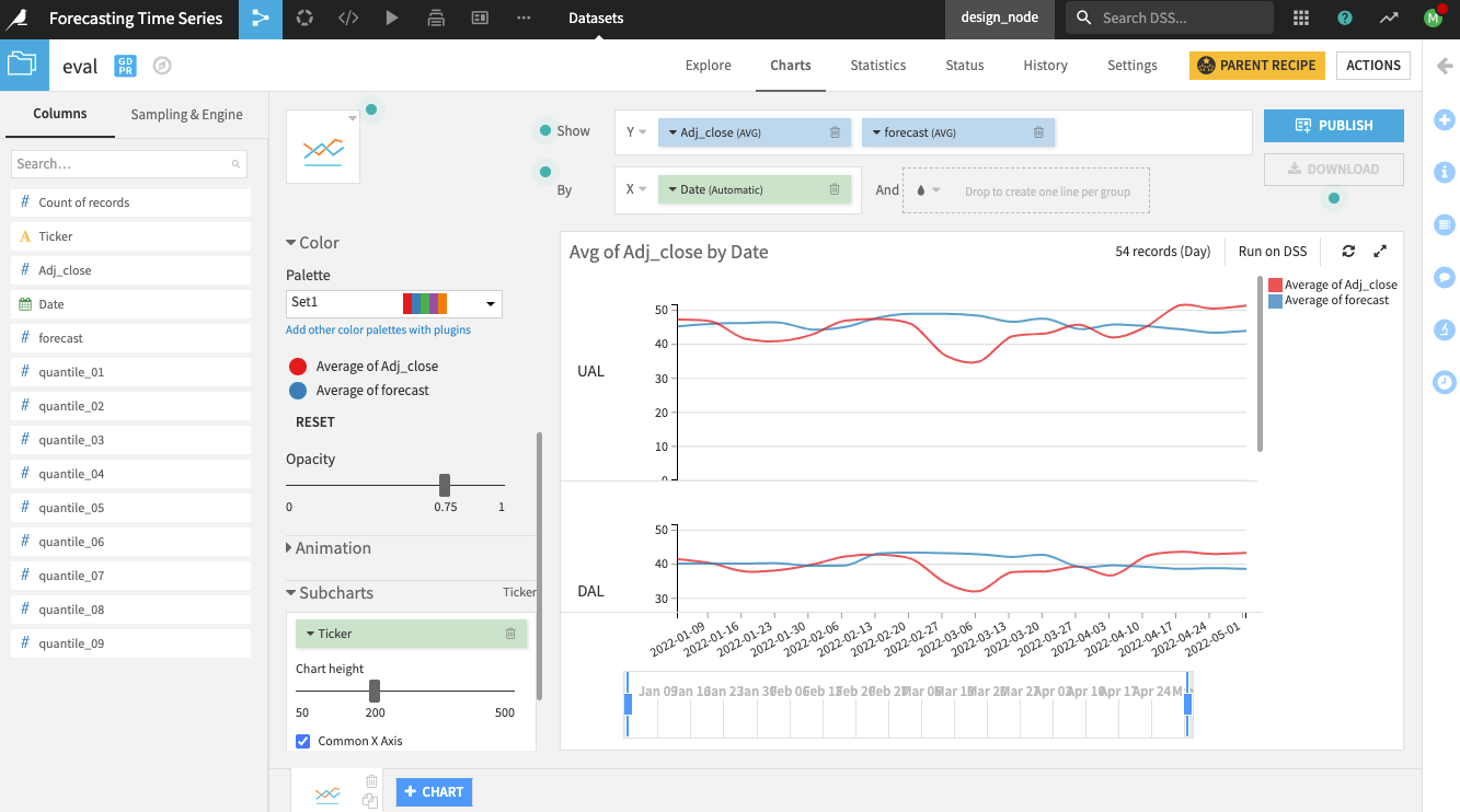
You can also create line charts on the dataset to compare the forecasts to the actual time series values.
In addition to the forecast values, you should also examine the associated metrics.
Open the metrics dataset to see one row of metrics per time series.

Score the Time Series Model
Finally, you can apply a Scoring recipe to the model to predict future values of the time series.
To apply the Scoring recipe to the time series model, you’ll use the airlines_stocks_prepared dataset as input. The Scoring recipe will use this input with the trained model to forecast future values of the time series (for dates after May 2, 2022).
To create the Scoring recipe,
Return to the Flow.
Click the model to select it from the Flow.
Click the Score recipe from the right panel.
Specify airline_stocks_prepared as the “Input dataset” to the recipe.
Name the output dataset
scored.Click Create Recipe.
Dataiku opens the recipe’s Settings page.
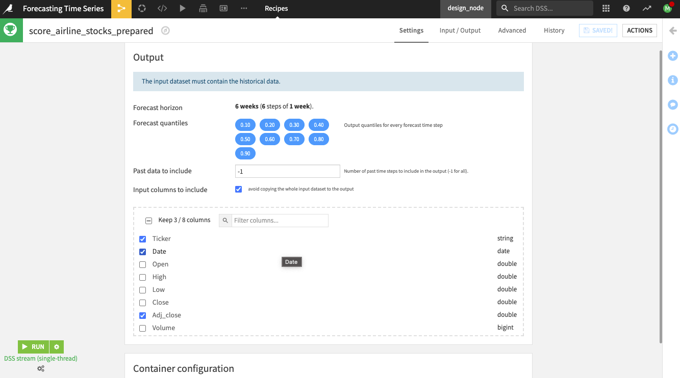
On the recipe’s Settings page, notice the following:
Dataiku alerts you that the “input dataset must contain the historical data.”
By default, the recipe uses a forecast horizon of six weeks (six steps in advance) since this was the model’s setting during training. Dataiku also outputs forecast values at different quantiles (the same ones used during training).
Specify the remaining settings as follows:
Specify the “Past data to include” as
52weeks.Keep the default checked box to avoid copying the whole input dataset to the output.
Keep the default selection of columns (Ticker, Date, and Adj_close) to include in the output.
Click Run to run the recipe. Wait for the run to finish.
Open the scored dataset.
Sort the scored dataset in descending order along the Date column to see the forecast values at the top of the dataset.
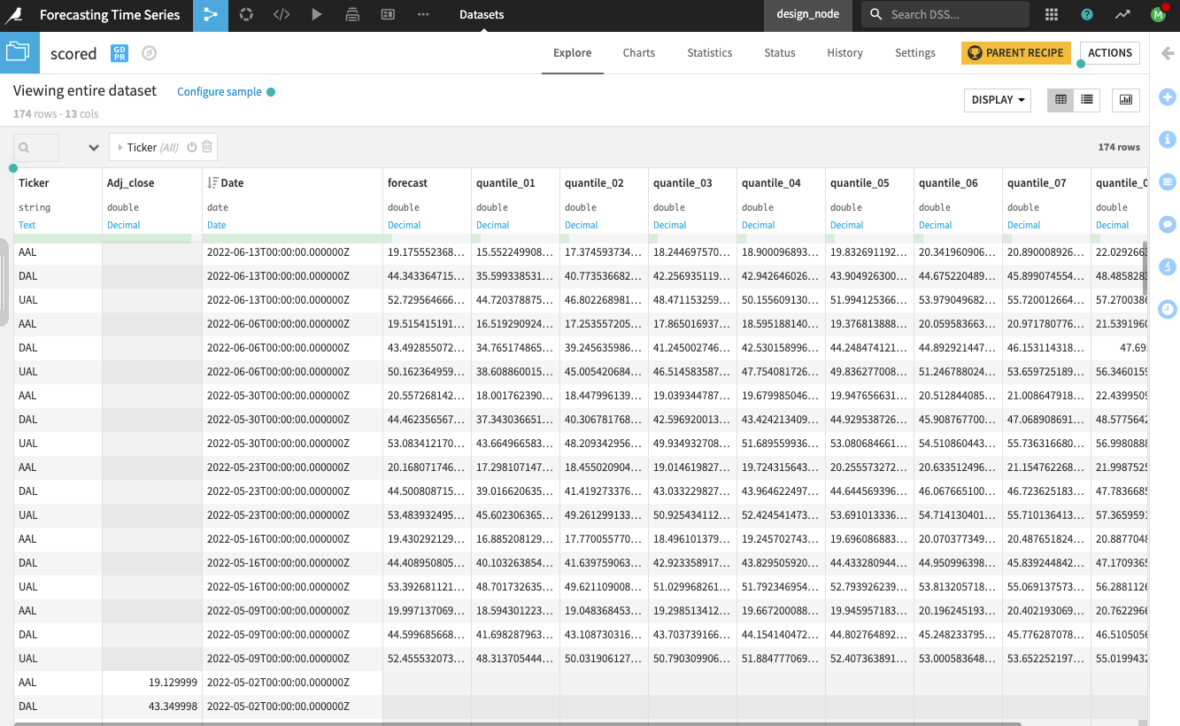
The recipe forecast values of the Adj_close alongside the quantiles for the next six weeks for each of the airline stocks.
Note
The product documentation provides more information on using the Scoring recipe with a time series model.
What’s Next?
Congratulations! You’ve taken your first steps toward modeling and forecasting time series data using Dataiku’s visual time series interface.
You can learn more about time series forecasting using the visual interface by checking out the product documentation on Time Series Forecasting.