The AI Lifecycle: Experiment
Having sufficiently explored and prepared the taxi fare data, the next stage of the AI lifecycle is to experiment with machine learning models.
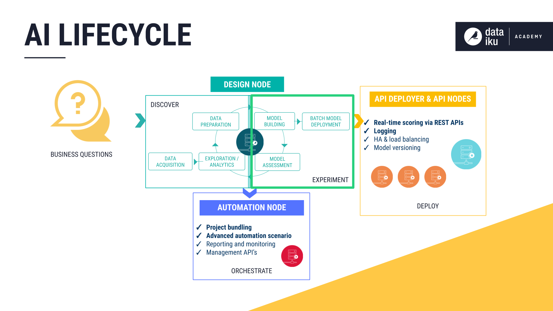
This experimentation stage encompasses two key phases: model building and model assessment.
Model building: Users have full control over the choice and design of a model — its features, algorithms, hyperparameters and more.
Model assessment: Tools such as visualizations and statistical summaries allow users to compare model performance.
These two phases work in tandem to realize the idea of Responsible AI. Either through a visual interface or code, building models with DSS can be transparently done in an automated fashion. At the same time, the model assessment tools provide a window into ensuring the model is not a black box.
Model Building
DSS is fully equipped to build models for both supervised (prediction) and unsupervised (clustering) learning tasks. After deciding on the type of task, users can decide if they wish to enter Expert mode and write a fully customized model or enter the Automated Machine Learning mode, where a visual interface guides model design.
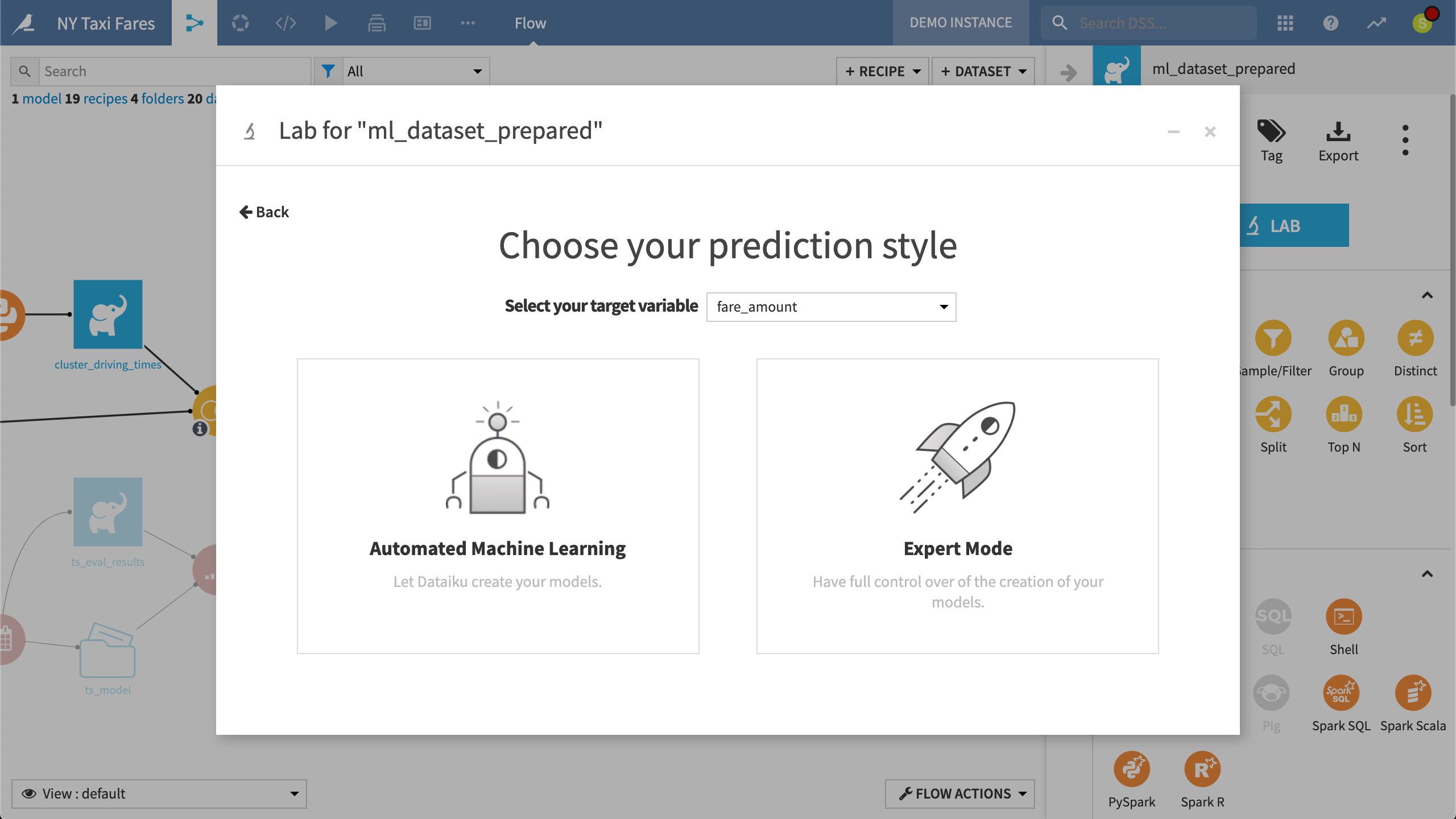
While in the Lab, after choosing a prediction task targeting the “fare_amount” variable, DSS presents the option of Automated Machine Learning or Expert Mode.
When building a visual model, users can choose a template instructing DSS to prioritize considerations like speed, performance, and interpretability. Having decided on the basic type of machine learning task, users retain full freedom to adjust the default settings chosen by DSS before training any models. These options include the split of the train and test set, the metric for which to optimize, what features to include, and what algorithms should be tested.
While trying to predict fares, the visual UI provides full control over what features to consider and how the algorithms should handle those features, including strategies for missing values and rescaling. Here, we can confirm that distance in kilometers is designated as a numeric input variable.
The automated machine learning capabilities allow users to train dozens of algorithms using a visual interface, while still leveraging state-of-the-art open source machine learning libraries, such as Scikit-Learn, MLlib, and XGBoost. In addition to these standard algorithms, users can also import custom Python models.
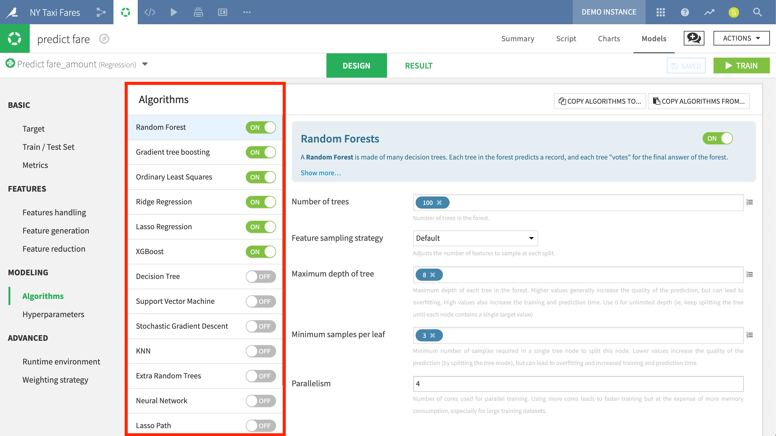
Here we are ready to train models using algorithms such as Random Forest and XGBoost. Users can control the parameters for each of these algorithms through the visual UI.
Furthermore, when training a prediction model on partitioned data, DSS is able to build partitioned (or stratified) models. Such a model is trained separately on each data partition, and so partition-level results can be compared against the overall model metrics. Partitioned models can lead to better predictions when relevant predictors for a target variable vary widely across partitions.
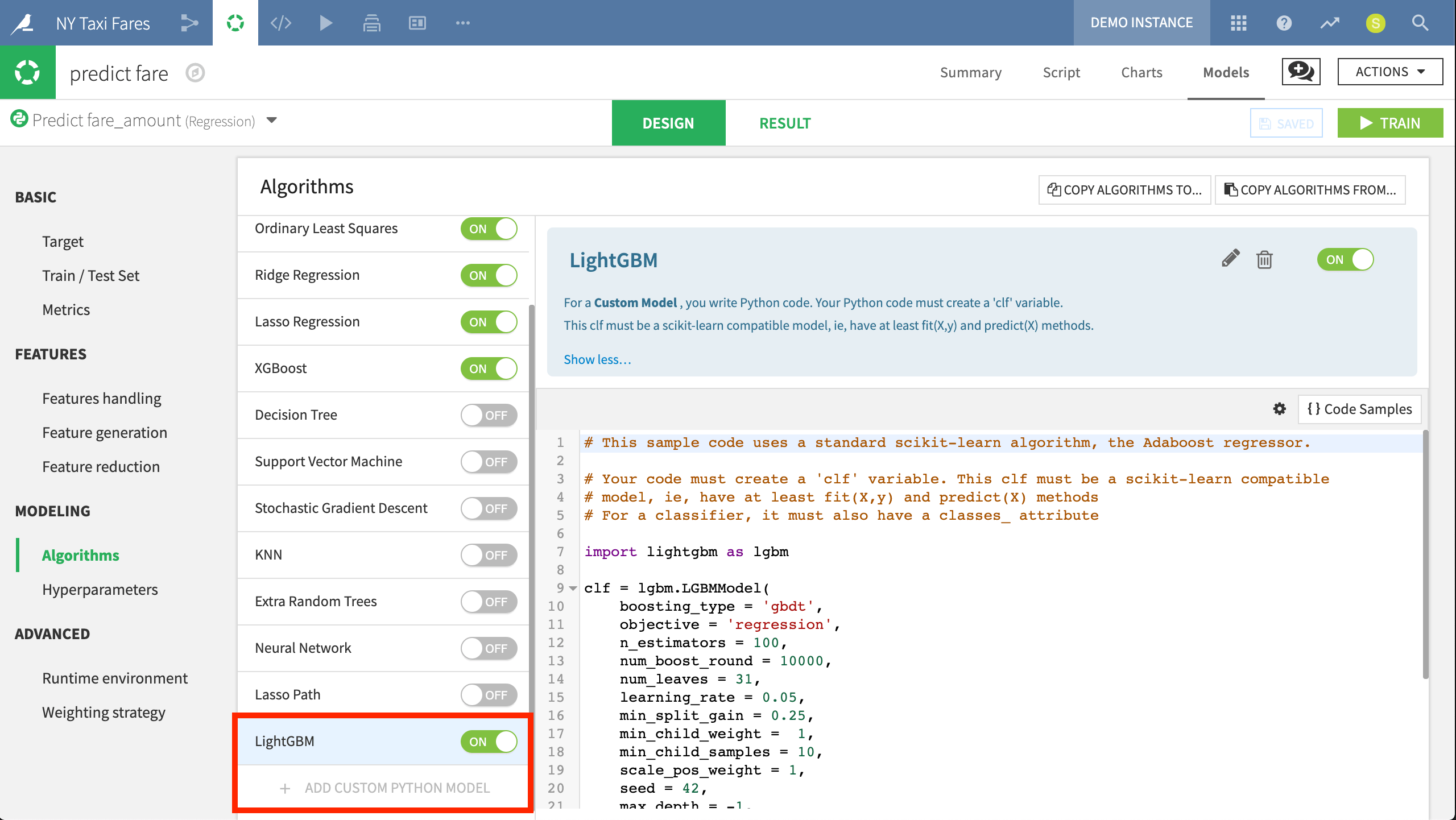
Here we have imported the LightGBM model into DSS. Originally developed by Microsoft, this algorithm performed slightly better than Random Forest and XGBoost in our example project.
Model Assessment
After having trained as many models as desired, DSS offers tools for full training management to track and compare model performance across different algorithms. DSS also makes it easy to update models as new data becomes available and to monitor performance across sessions over time.
In the Result pane of any machine learning task, DSS provides a single interface to compare performance in terms of sessions or models, making it easy to find the best performing model in terms of the chosen metric.
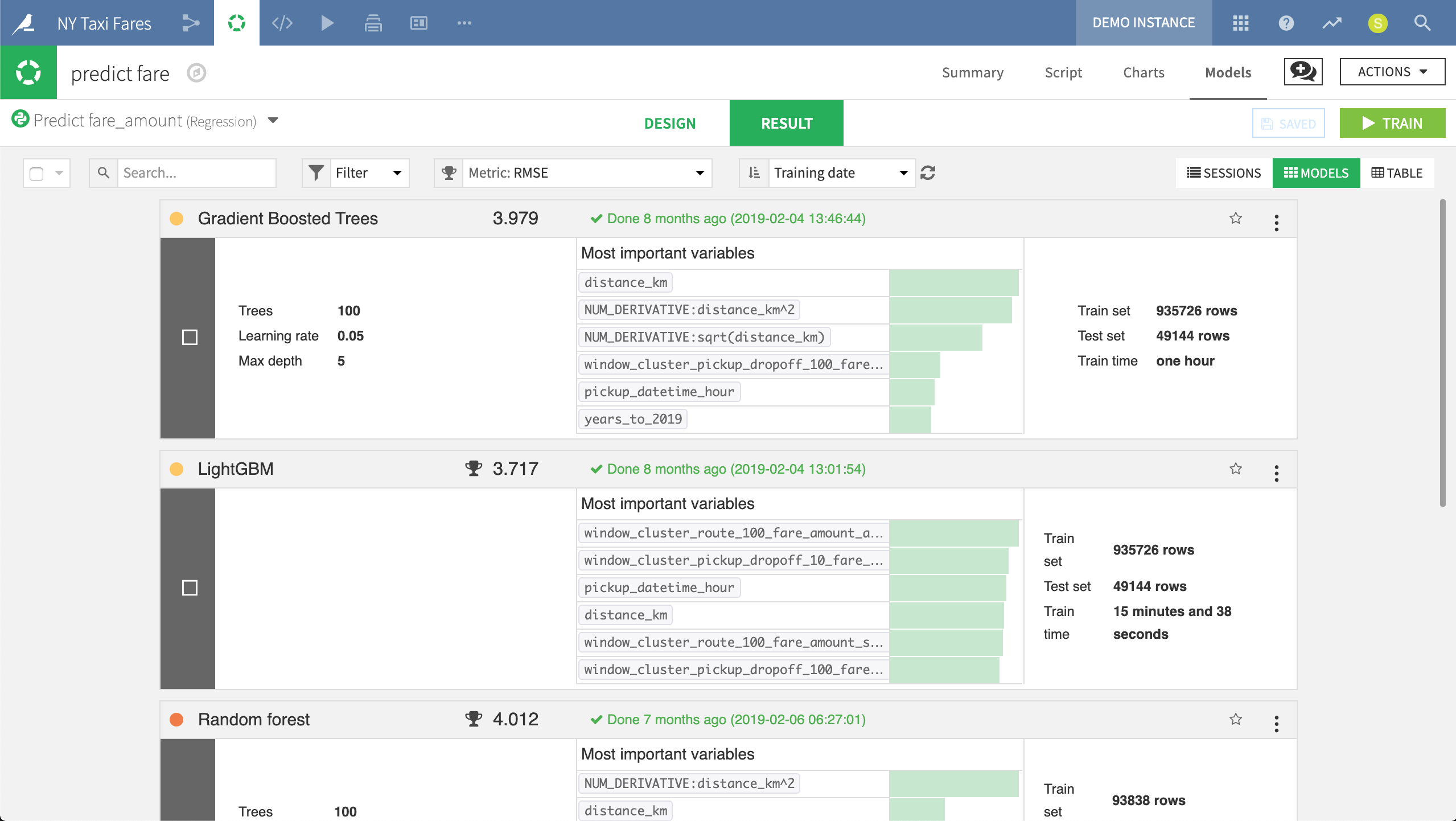
Here we can compare the performance of various models and see at a glance how they differ in terms of the most important variables. In this case, LightGBM, an imported model built in Python, had the lowest Root Mean Square Error (RMSE).
Just clicking on any model produces a full report of tables and visualizations of performance against a range of different possible metrics.
Here we can review the report of the Light GBM model. Each tab in the left panel provides a different insight into the model’s interpretation, performance or other information.