R Markdown Reports in Dataiku DSS¶

Overview¶

R Markdown is an R package to create fully reproducible, print-quality documents that incorporate narrative text and code to produce elegant output that can be shared on dashboards or delivered in a variety of static formats for offline reading.

It is an example of literate programming as it weaves together natural language with source code.

In this brief tutorial, we’ll create a simple R Markdown report in Dataiku DSS. The final output can be viewed on the Dataiku gallery.

Technical Requirements¶

A proper installation of R on the server running DSS.
- See the reference documentation if you do not have the R integration installed.
An existing R code environment including the ggplot2 and magrittr packages, in addition to the required dplyr and dataiku packages
- Instructions for creating an R code environment can be found in the reference documentation.
An installation of pandoc, in order to download reports as PDFs, with the adjustbox, collectbox, ucs, collection-fontsrecommended, and titling LaTeX packages.

Supporting Data¶

The Orders_by_customer dataset.
- This dataset can be found in the project DSS Tutorials > Automation > Deployment.
- Alternatively, directly download the data here in a new blank project.

Creating A New R Markdown Report¶

From the Deployment tutorial or the new blank project if directly downloading the data, create a new empty R Markdown report:

In the Code menu (</>) of the top navigation bar, select RMarkdown Reports.
Click “+ New Report” or “+ Create Your First Report”.
Choose “Empty document” and type a name for the report, in this case Haiku T-Shirt Analytics.

You will be redirected to the R Markdown editor.

The R Markdown Editor¶

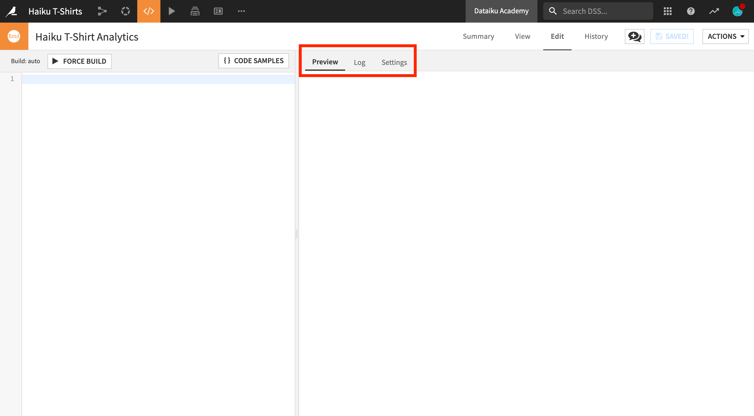
The R Markdown editor is divided into two panes.

The left pane allows you to see and edit the markdown (including code) underlying the report.

The right pane gives you several views on the report.

The Preview tab allows you to write and test your markdown in the left pane while having immediate visual feedback in the right pane. At any time you can save or reload your current markdown by clicking on the Save button.
The Log is useful for troubleshooting problems.
Settings allows you to set the output format of the preview. You can also set the code environment, if you want it to be different from the project default.

Writing An R Markdown Report¶

Let’s build the markdown and code behind the report. In this section, we’ll add three types of content:

Metadata inside a YAML header, wrapped by ---
R code chunks, wrapped by ```
Narrative text with simple markdown formatting

Defining the Document Metadata¶

Start with the YAML header, demarcated by three dashes, ---, to define document metadata.

In the left pane, insert the following code to define document properties, including the title, author name, date, and how to handle certain types of output.

The report date specification uses R code to insert the current system date.
When generating PDF output for this report, it should include a table of contents.

---
title: "Haiku T-Shirt Analytics"
author: "Dataiku Learn"
date: "`r format(Sys.Date())`"
output:
    pdf_document:
        toc: true
---

This YAML header defines only a few properties, but it can control many options such as the formatting of sections, figures and tables.

Importing the Necessary Packages¶

In an R Markdown document, three backticks demarcate the beginning and end of a code chunk.

In the left pane, insert the following code chunk to import the R packages that will be used to generate the report output.

```{r echo=FALSE, warning=FALSE, message=FALSE}
# Pull the necessary libraries
library(dataiku)
library(magrittr)
library(ggplot2)
library(dplyr)
```

Each code chunk specifies the language (in this case, R) and additional parameters that apply to that code chunk. These parameter settings will not include the code itself in the final output, nor print any warnings or messages.

Report Introduction and Data Import¶

The third type of content in an R Markdown report is narrative text (markdown).

In the left pane, insert the following code chunk and line of text.

```{r echo=FALSE, warning=FALSE, message=FALSE}
# Read the Dataiku dataset we want to use
df <- dkuReadDataset("Orders_by_customer", samplingMethod="head", nbRows=1000000)
```

This report is prepared for the executives of the Haiku T-Shirt company to apprise them of the current state of customer analytics.

It uses the dkuReadDataset() function to read the Orders_by_customer dataset in the same way an R code recipe would. Outside of the code chunk, text forms the body of the report.

Basic Reporting on Customer Location¶

Now let’s build the first main section of the report.

In the left pane, insert the following block of code and text:

# Customers by Country

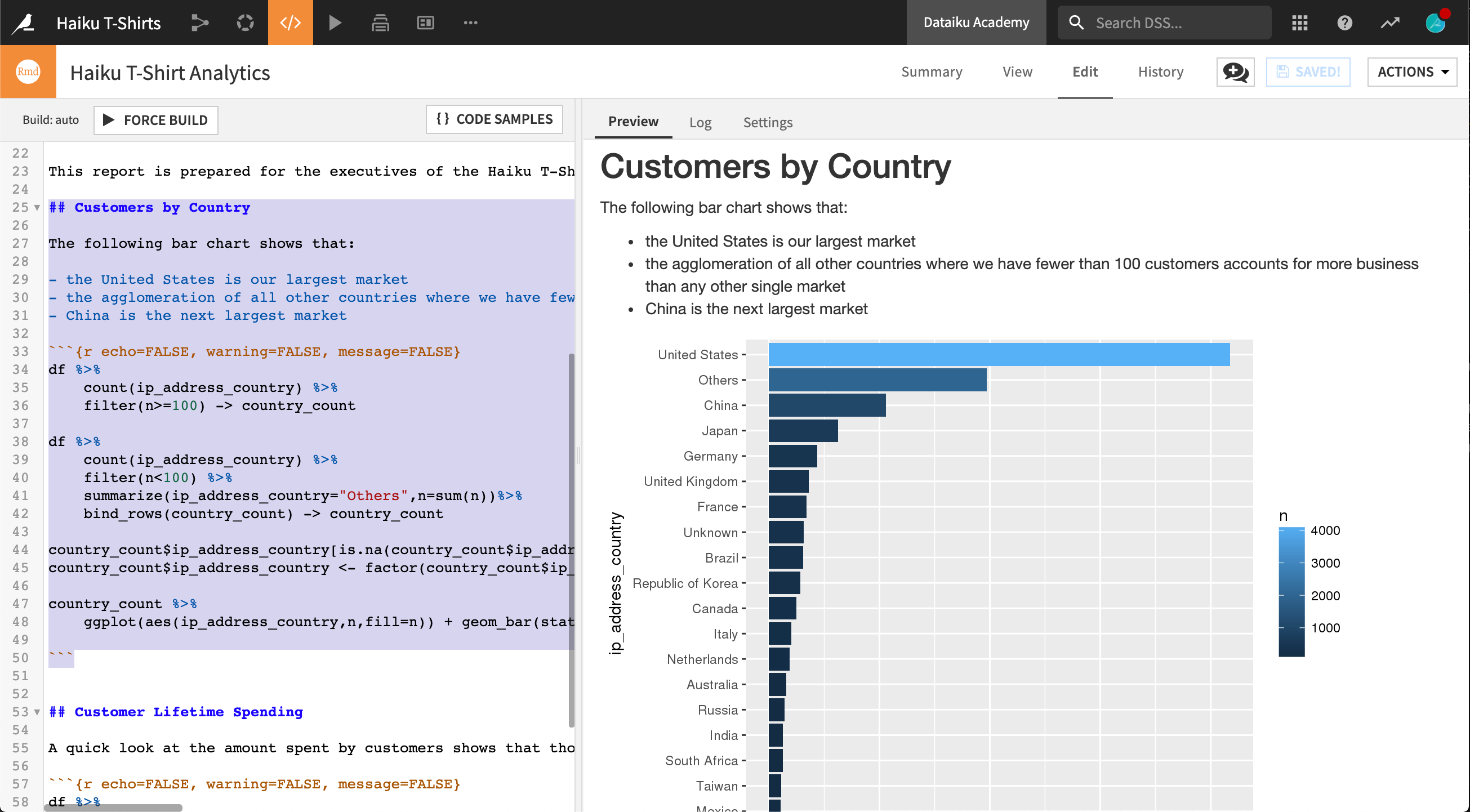
The following bar chart shows that:

- the United States is our largest market
- the agglomeration of all other countries where we have fewer than 100 customers accounts for more business than any other single market
- China is the next largest market

```{r echo=FALSE, warning=FALSE, message=FALSE}
df %>%
    count(ip_address_country) %>%
    filter(n>=100) -> country_count

df %>%
    count(ip_address_country) %>%
    filter(n<100) %>%
    summarize(ip_address_country="Others",n=sum(n))%>%
    bind_rows(country_count) -> country_count

country_count$ip_address_country[is.na(country_count$ip_address_country)] <- "Unknown"
country_count$ip_address_country <- factor(country_count$ip_address_country,
                                        levels=country_count$ip_address_country[order(country_count$n)])

country_count %>%
    ggplot(aes(ip_address_country,n,fill=n)) +
      geom_bar(stat="identity") +
      coord_flip()

```

Now let’s analyze this block in detail, piece by piece:

Outside of a code chunk, the hashtag, #, is a markdown indication for a new heading.
The text that explains the chart uses the - markdown to create a bulleted list.

../../../_images/rmd-customers-by-country.png

The R code produces the plot above in several steps:

Process the raw data frame to count the number of customers in each country, filtering out all countries with fewer than 100 customers, and saving to a country_count data frame.

df %>%
  count(ip_address_country) %>%
  filter(n>=100) -> country_count

Count the total number of customers across countries with fewer than 100 customers each, and add them as an extra row in the country_count data frame.

df %>%
  count(ip_address_country) %>%
  filter(n<100) %>%
  summarize(ip_address_country="Others",n=sum(n))%>%
  bind_rows(country_count) -> country_count

Recode the NA values for customers whose country is unknown to the string “Unknown”; then reorder the factor levels of the column ip_address_country so that they are organized in descending order from the country with the most customers to the one with the least.

country_count$ip_address_country[is.na(country_count$ip_address_country)] <- "Unknown"
country_count$ip_address_country <- factor(country_count$ip_address_country,
                                      levels=country_count$ip_address_country[order(country_count$n)])

Finally, create the bar chart of number of customers per country, with the coordinate axis flipped so that the bars are horizontal rather than vertical.

country_count %>%
  ggplot(aes(ip_address_country,n,fill=n)) +
    geom_bar(stat="identity") +
    coord_flip()

Reporting on Customer Lifetime Spending¶

Now build the second graphic. In the left pane, insert the following markdown and code.

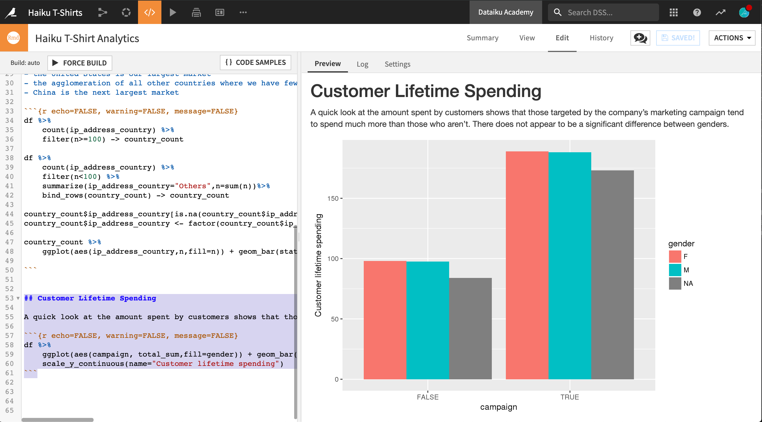
The R code in this section produces another bar chart, showing the total amount spent by customers, broken down by gender and whether they are part of the company’s marketing campaign.

# Customer Lifetime Spending

A quick look at the amount spent by customers shows that those targeted by the company's marketing campaign tend to spend much more than those who aren't.  There does not appear to be a significant difference between genders.

```{r echo=FALSE, warning=FALSE, message=FALSE}
df %>%
    ggplot(aes(campaign, total_sum,fill=gender)) +
    geom_bar(stat="summary",fun.y="mean",position="dodge") +
    scale_y_continuous(name="Customer lifetime spending")
```

../../../_images/rmd-customer-lifetime-spending.png

Publishing An R Markdown Report¶

When you are done with editing, there are a number of options for distributing your report.

Publish on a dashboard from the Actions dropdown at the top-right corner of the screen.
Download to your local filesystem in one of a variety of formats, again from the Actions dropdown.
Email as part of an automation scenario.

What’s next¶

Congratulations! Using Dataiku DSS, you have created an R Markdown report.

You can examine a completed version of this report on the Dataiku gallery.

For further inspiration on what is possible in R Markdown reports, see the R Markdown gallery (external).