Geographic Processing with Dataiku DSS

This tutorial demonstrates many of the visual geographic processors available in Dataiku DSS.

Workflow Overview

Using the data on French post offices from the Mapping in DSS lesson and the familiar Haiku T-Shirt customer data used in many examples, this tutorial reviews processors that:

• Create GeoPoints from lat/lon coordinates

• Extract lat/lon coordinates from GeoPoints

• Resolve IP addresses to geographic information like country and coordinates

• Calculate distance between two geographic points

• Perform a geographic nearest-neighbor join between two datasets with geographic coordinates.

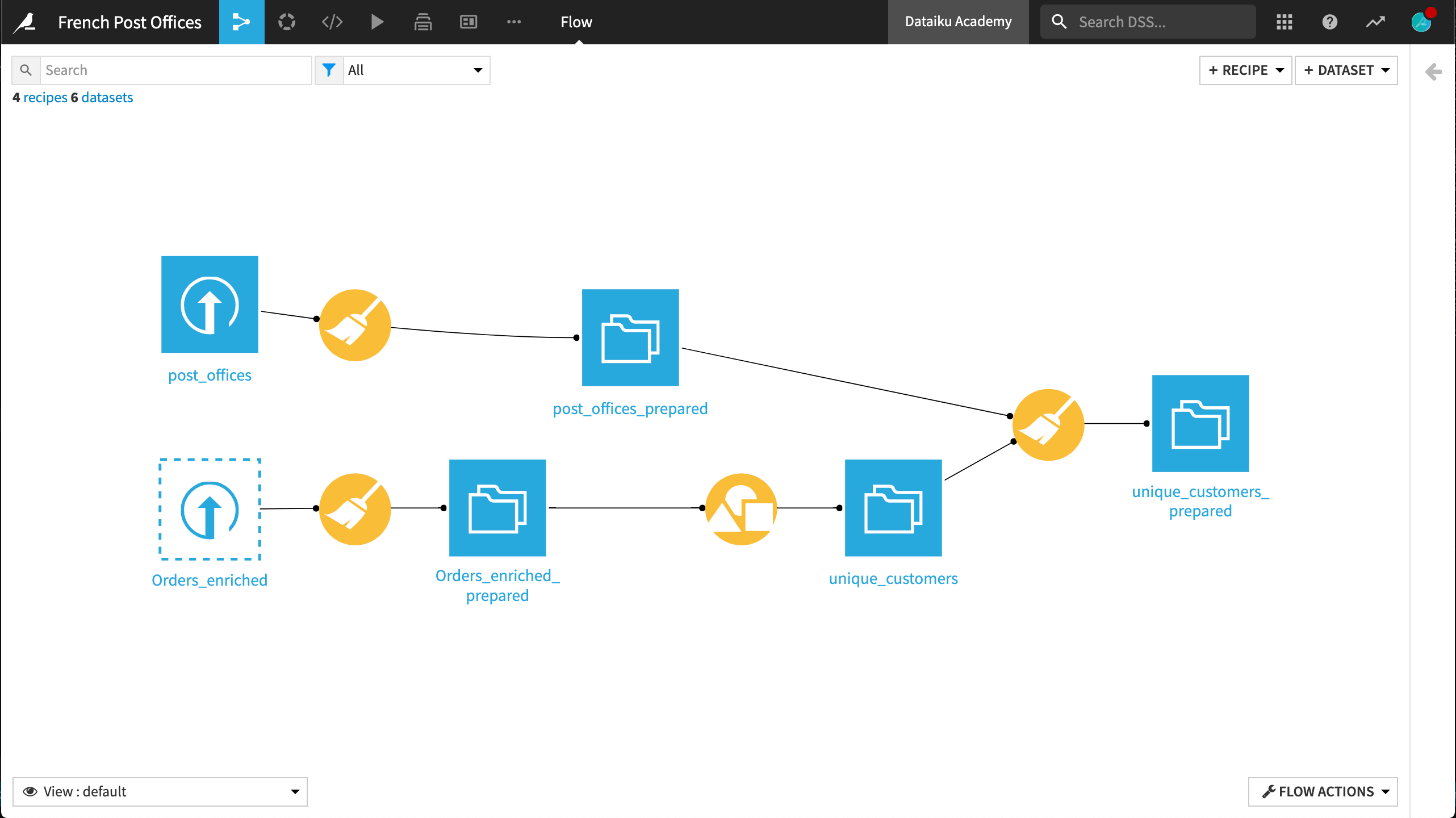
By the end of this brief walkthrough, your workflow in Dataiku DSS should mirror the one below. Moreover, the completed project can be found in the Dataiku gallery.

Supporting Data

The data in this tutorial come from two sources:

• The first dataset is the post_offices_prepared, found following the data preparation steps in the Mapping in DSS tutorial .

• The second dataset, Orders_enriched, comes from the fictional retailer, Haiku T-Shirts. It can be exported from the Automation tutorial or can be downloaded directly as a CSV file here.

Creating GeoPoints

Resume the project created in the Creating Maps in DSS without code lesson.

Recall that this lesson used the Create GeoPoint from lat/lon processor in the Prepare recipe, compute_post_offices_prepared .

This visual processor takes two columns of latitude and longitude coordinates as input and produces a GeoPoint ready for mapping and other spatial analysis.

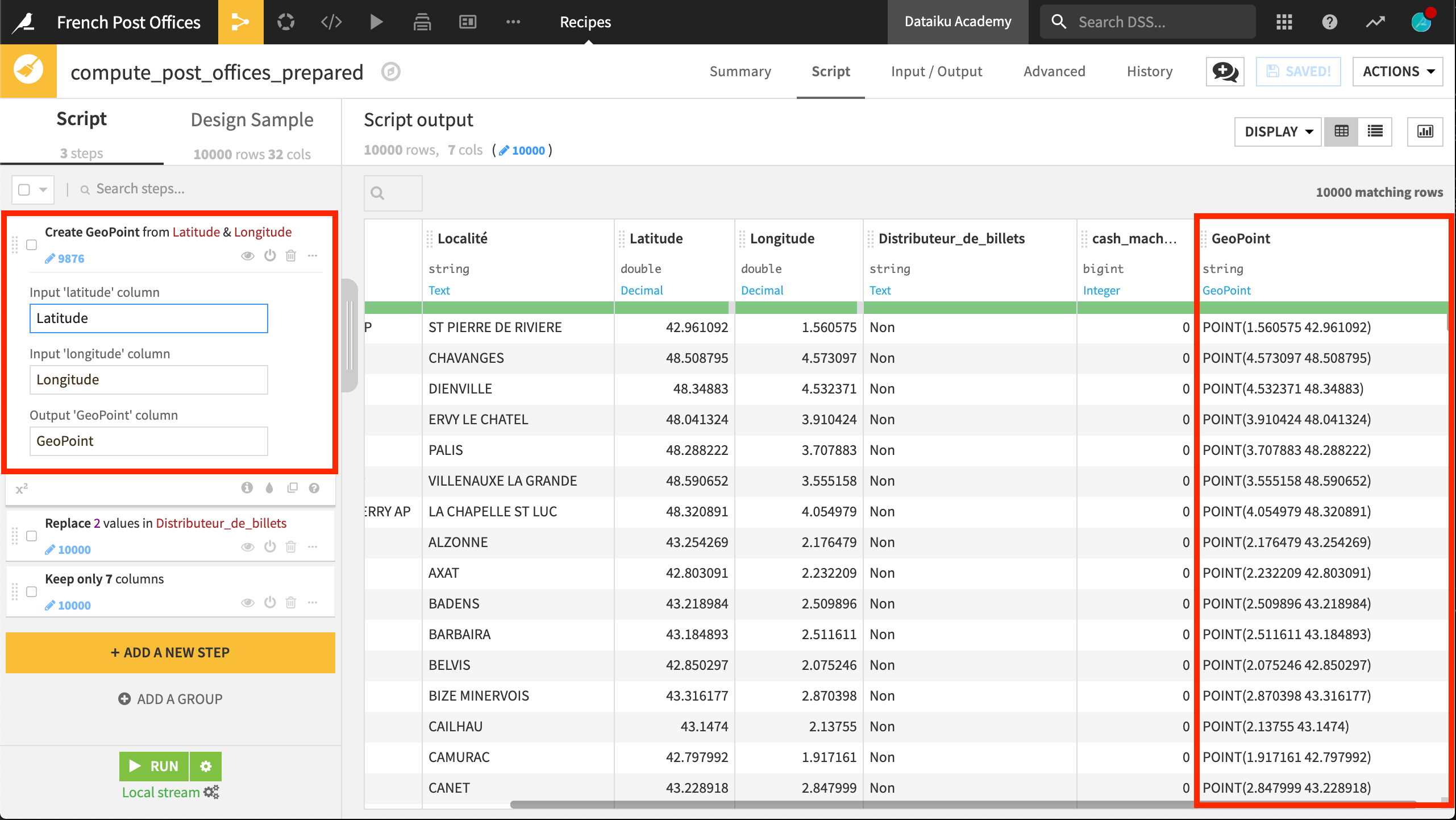
If not yet having already done so, deploy the visual analysis script to the Flow, creating the output dataset post_offices_prepared.

Resolving IP Addresses

In the previous tutorial, we successfully mapped the location of post offices in France. Now we want to compare those locations to the locations of our French customers.

In the same project, upload the Orders_enriched dataset from the Haiku T-Shirt retailer.

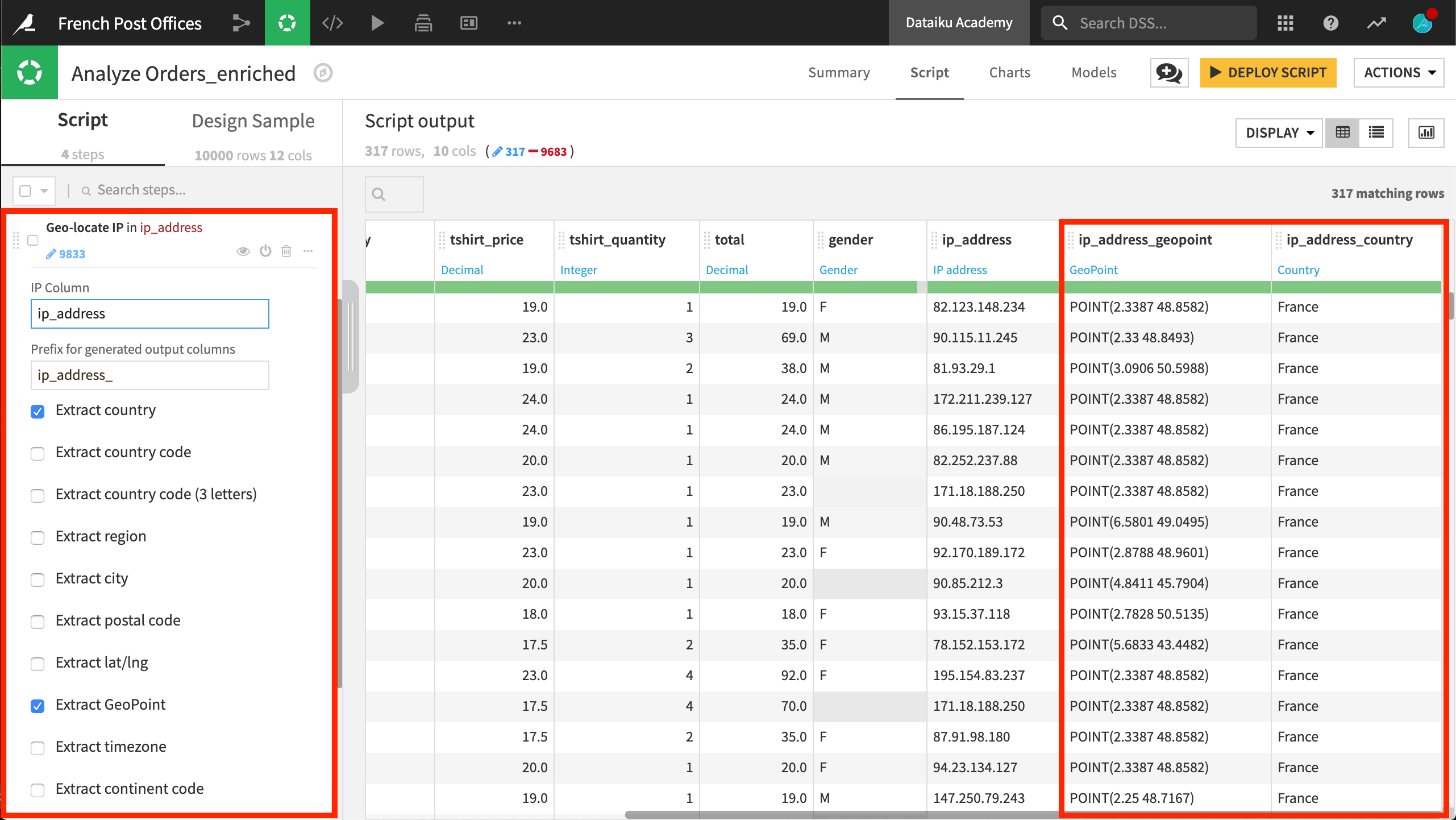
This data includes information on orders made by customers, including the IP address of those customers. From this IP address, we can use the Resolve GeoIP visual processor to extract a geographic location for each customer.

• After uploading the dataset, create a new visual analysis in the Lab.

• To simplify the data wrangling, remove five columns we won’t need: order_date, pages_visited, birthdate, user_agent, and campaign.

• Using the Formula processor, create a new column total using the expression tshirt_price * tshirt_quantity.

• Use the Resolve GeoIP processor on the ip_address column, extracting the country and GeoPoint as new columns. Use ip_address_ as the prefix for generated output columns.

• Using one of these new columns, it’s now easy to keep only rows where ip_address_country is France.

Deploy this Script to the Flow, producing the output dataset Orders_enriched_prepared.

Mapping Unique Customers

The Resolve GeoIP processor produced a location for each customer. The dataset, however, could use some cleaning. Before mapping, let’s perform a simple Group By recipe to get a dataset of unique customers.

• From the Orders_enriched_prepared dataset, initiate a Group By recipe.

• Choose to group by customer_id and name the output dataset unique_customers.

• In the Group step, for Per Field Aggregations, choose the Sum of total, the First of gender, and the First of ip_address_geopoint.

• In the Output step, remove the “_first” from the gender and ip_address_geopoint columns for clarity,.

• Run the recipe.

We can visualize our progress with a quick map of the results.

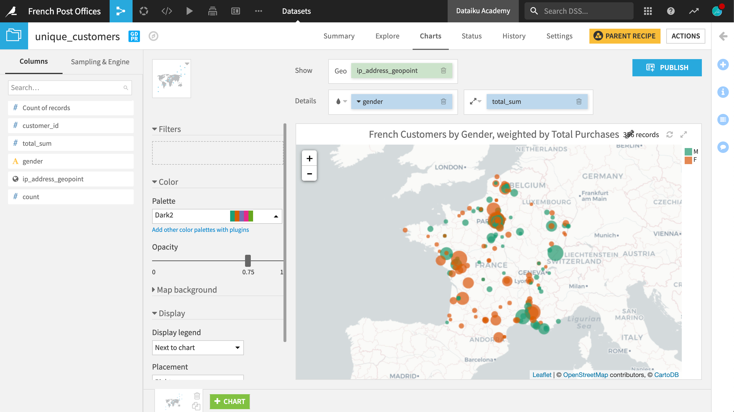
• On the Charts tab of the unique_customers dataset, create a Scatter Map.

• Drag ip_address_geopoint to the Geo field, gender to the color droplet, and total_sum to the base radius field.

Now we have an interactive map of all customers in France colored by gender and scaled according to the total sum of all their purchases.

Calculating Distance

To begin analyzing our potential shipping costs, let’s simply calculate the distance from the office to each customer.

• From the unique_customers dataset, create a Prepare recipe.

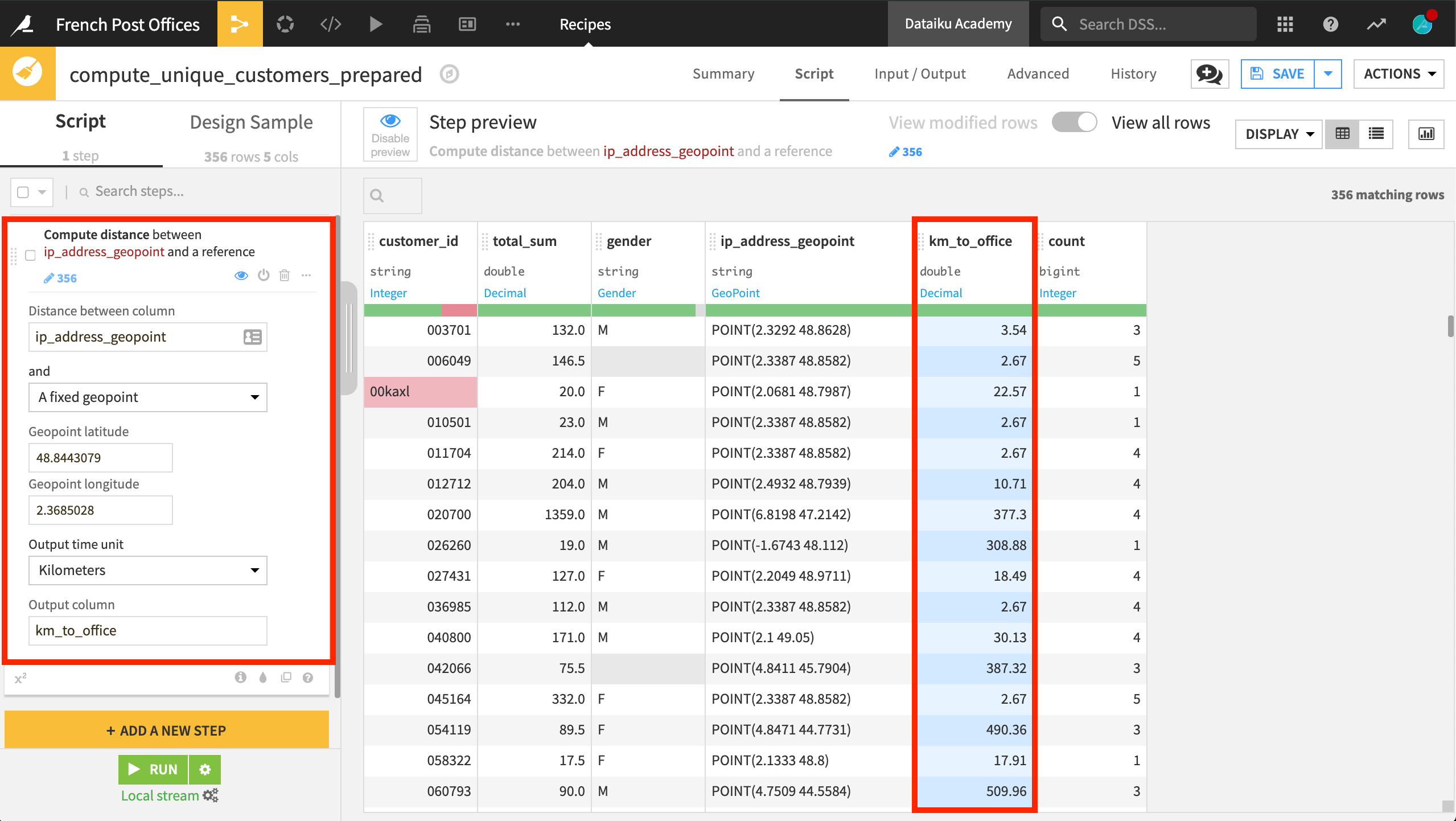
• Use the Compute distance between geopoints processor on the ip_address_geopoint column.

  • This processor will compute distance between a fixed geopoint or another geopoint column. Choose a fixed geopoint with lat/lon coordinates of 48.8443079 and 2.3685028, respectively.

  • Select kilometers as the output unit and name the column km_to_office.

Using the Analyze tool, we can see that the km_to_office column has an extremely right-skewed distribution, with the vast majority of customers less than 20 kilometers away and small numbers of customers hundreds of kilometers away.

Geo-Joining Spatial Datasets

In order to ease our shipping costs, perhaps we could explore collaboration with the network of post offices. We can use the Geo-join processor to find the nearest post office to every customer.

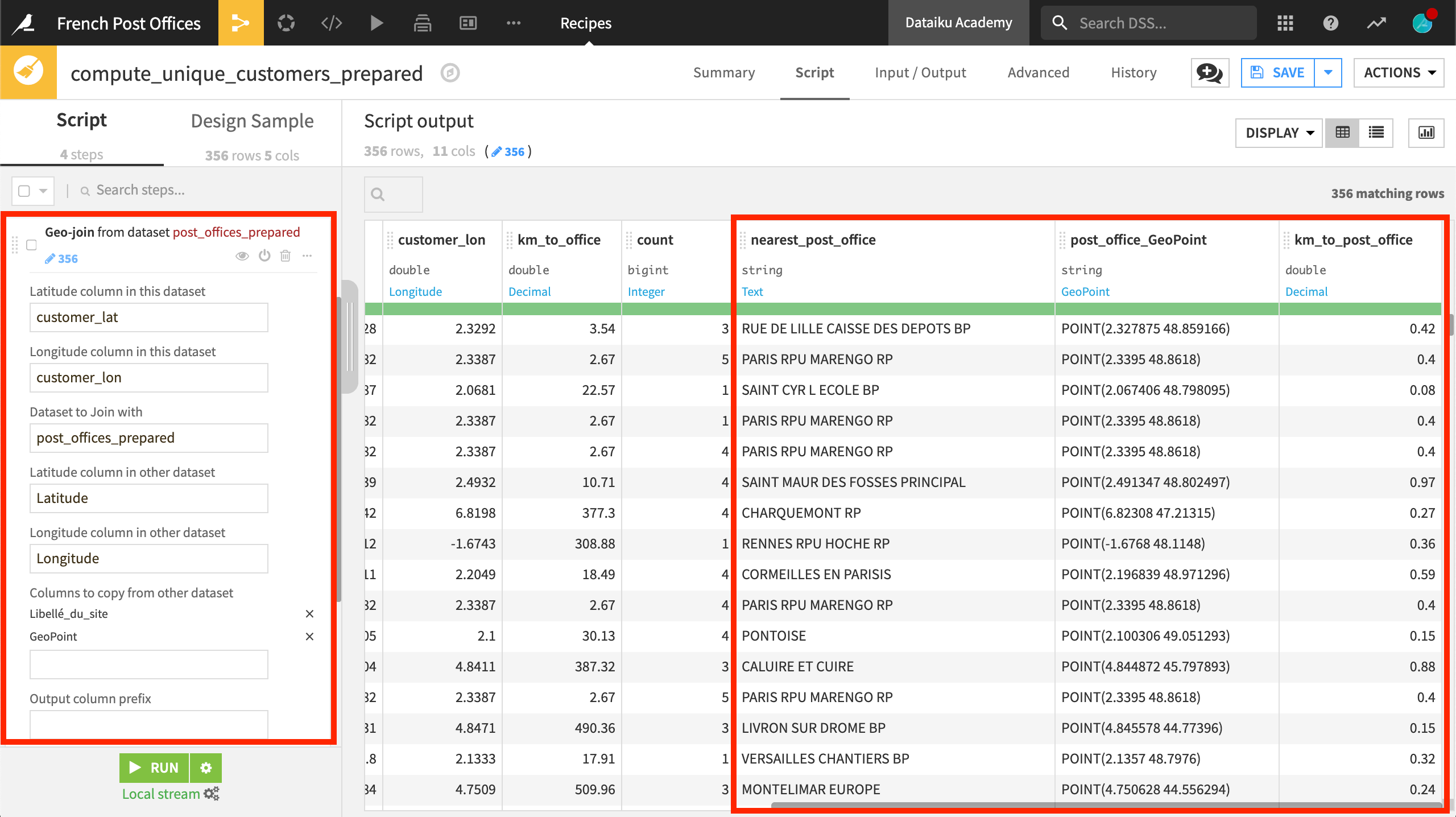
• In same Prepare recipe (compute_unique_customers_prepared), use the Extract lat/lon from GeoPoint processor on the ip_address_geopoint column to produce two output columns: customer_lat and customer_lon.

• Use the Geo-join processor to match the nearest post office to each customer.

  • customer_lat and customer_lon are the columns from “this” dataset. They need to be joined with the Latitude and Longitude columns from the post_offices_prepared dataset.

  • Additionally, copy the columns Libellé_du_site and GeoPoint.

• In another step, rename the new columns for clarity:

  • Libellé_du_site to nearest_post_office

  • GeoPoint to post_office_GeoPoint

  • join_distance to km_to_post_office.

• Run the recipe.

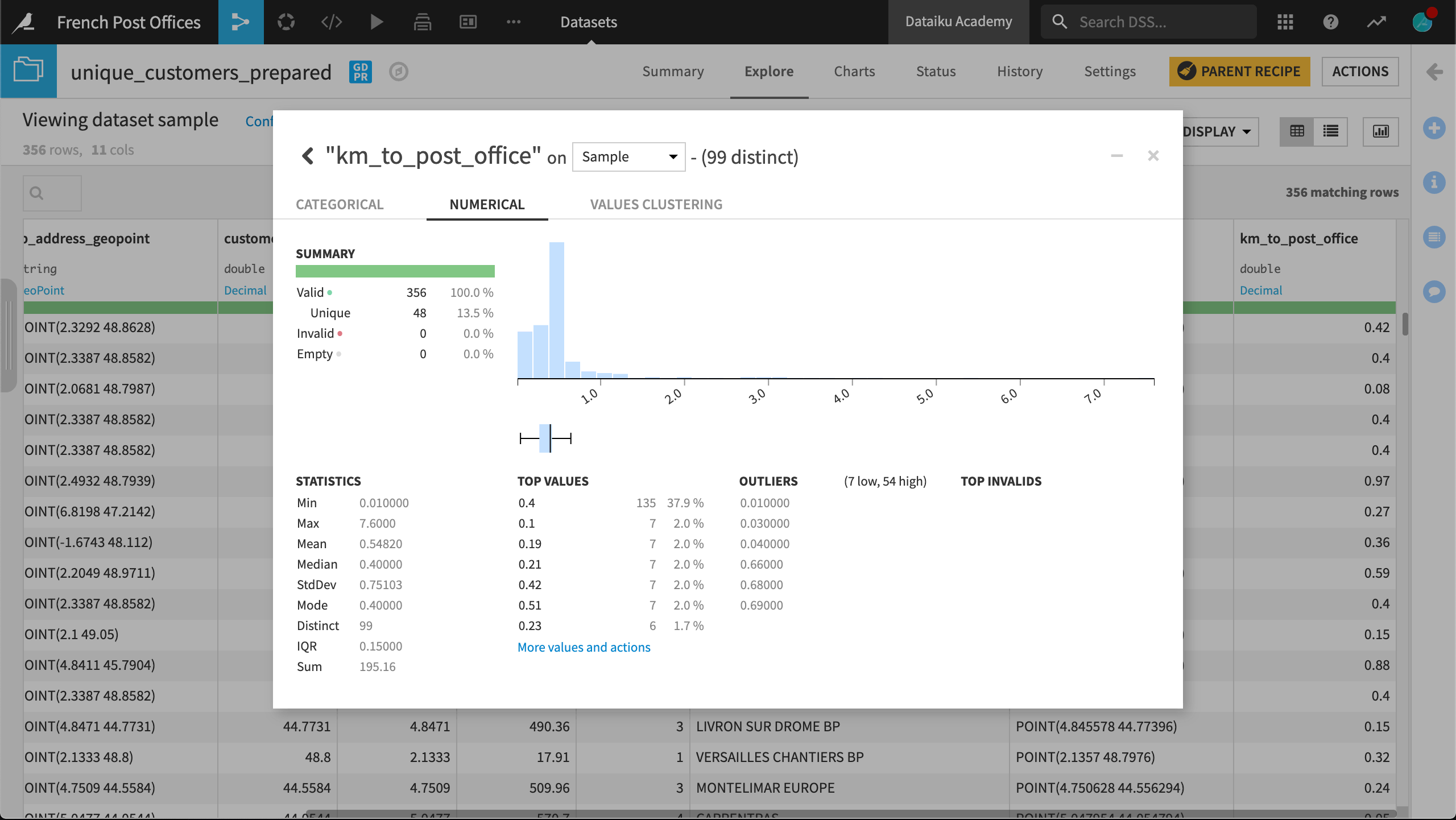
In the output dataset, unique_customers_prepared, we can use the Analyze tool to examine the most common post offices and the distribution of the distance to the nearest post office.

• It seems nearly 40% of customers share the same nearest post office.

• Nearly all customers have a post office within 1 kilometer (according to their IP address).

What’s Next?

Congratulations! You used a range of different visual geographic processors to determine the distance between customers and their nearest post office.

Review a read-only version of this project in the Dataiku gallery.

More information about geographic processing in DSS can be found in the reference documentation.