Hands-On: Handling Text Features for ML

In the previous hands-on lesson, we applied simple text cleaning operations like normalization, stemming, and stopwords removal to improve a model that classifies positive and negative movie reviews.

We have done some text cleaning and basic feature engineering, but another tool is adjusting how Dataiku DSS handles those features when building models.

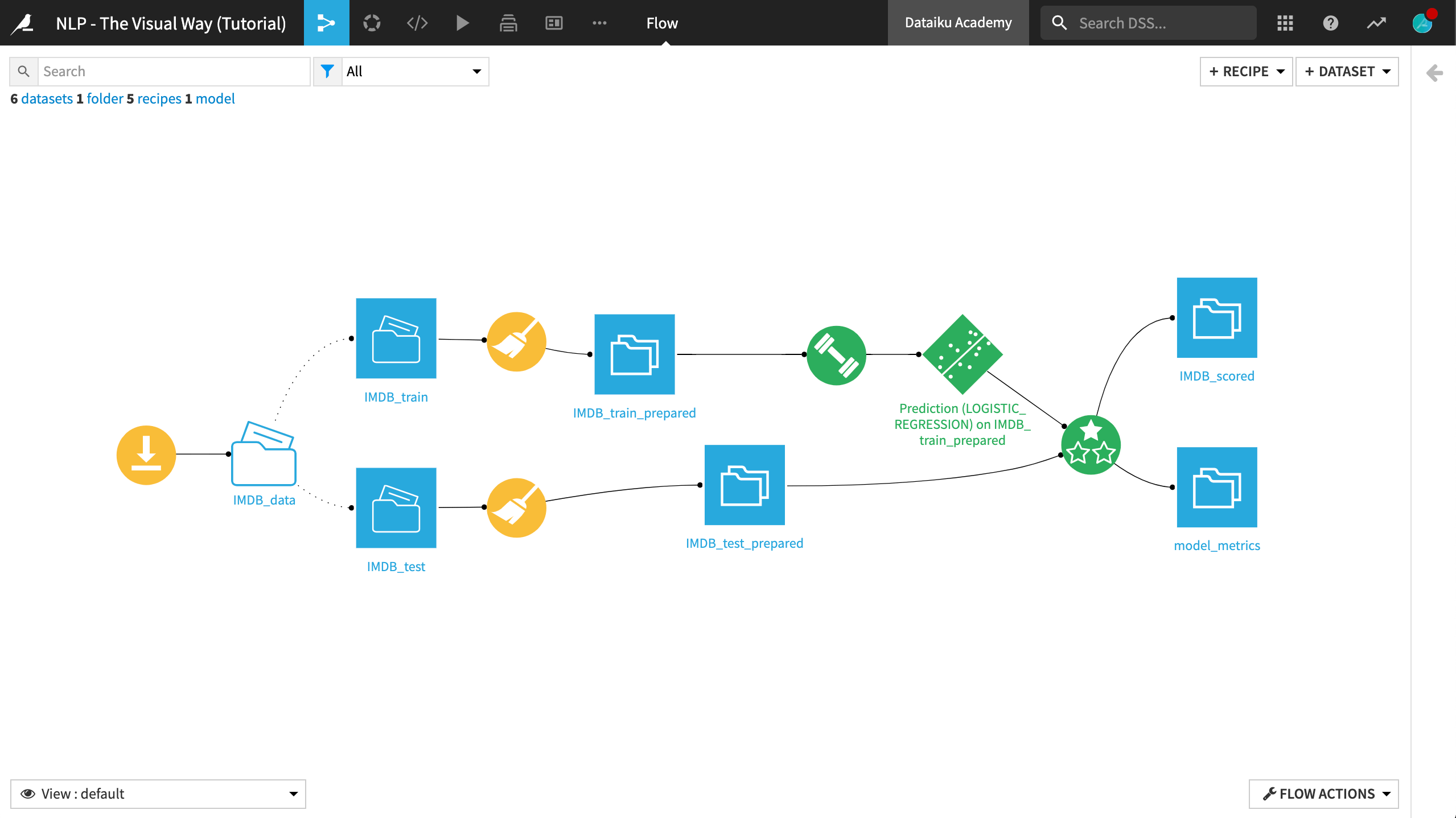
In this lesson, we’ll experiment with different text handling methods and evaluate the performance of our model against a test dataset. When finished, the final Flow should resemble the image below.

Vectorization Methods

Return to the modeling task on the IMDB_train_prepared dataset. In the Features handling pane of the Design tab:

• Adjust the Text handling method from the default “Tokenize, hash and apply SVD” to “Counts vectorization”.

• Click Train.

• Name the session count vec.

• Accept the message to drop existing sets and recompute new ones.

• Accept the warning message for unsupported sparse features.

• Click Train.

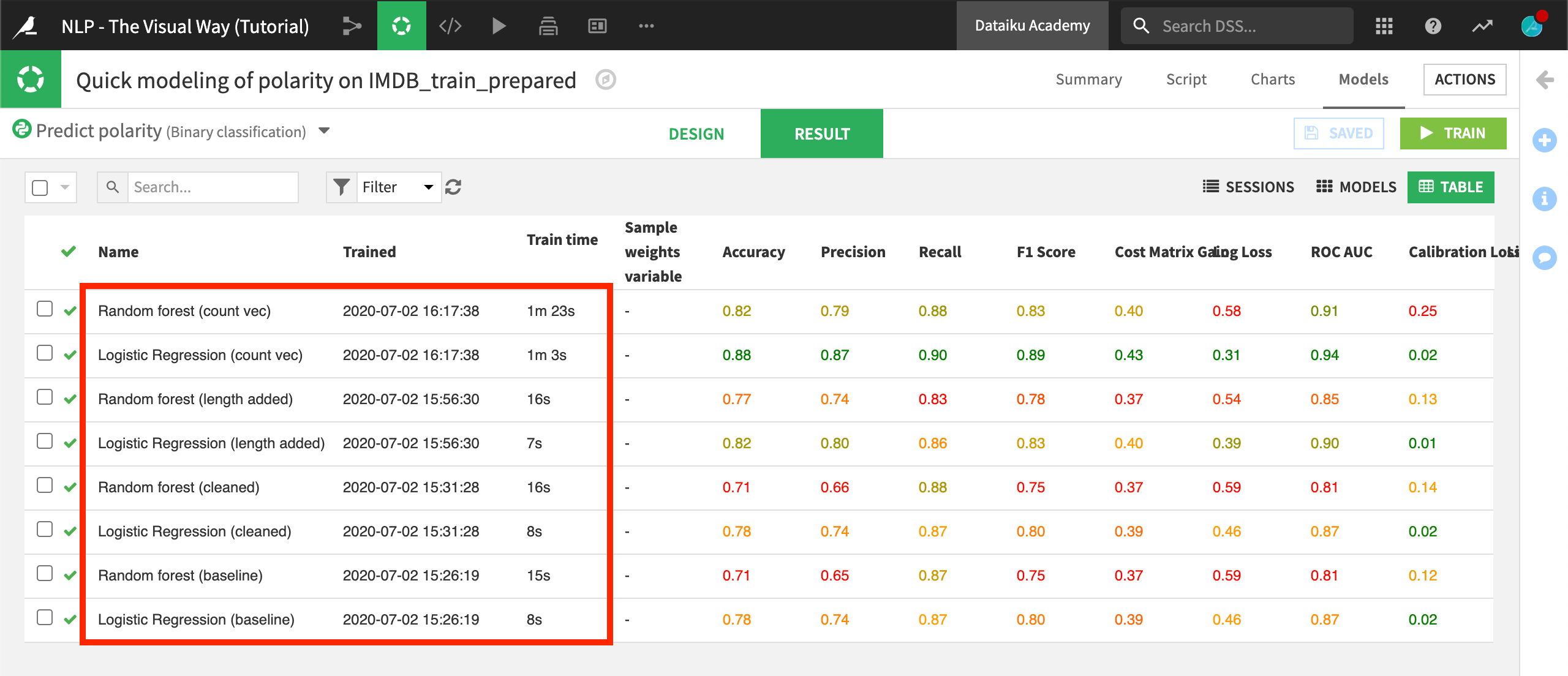
When the fourth session finishes training, we can see that the count vectorization models have a considerable edge over the term hashing + SVD predecessors.

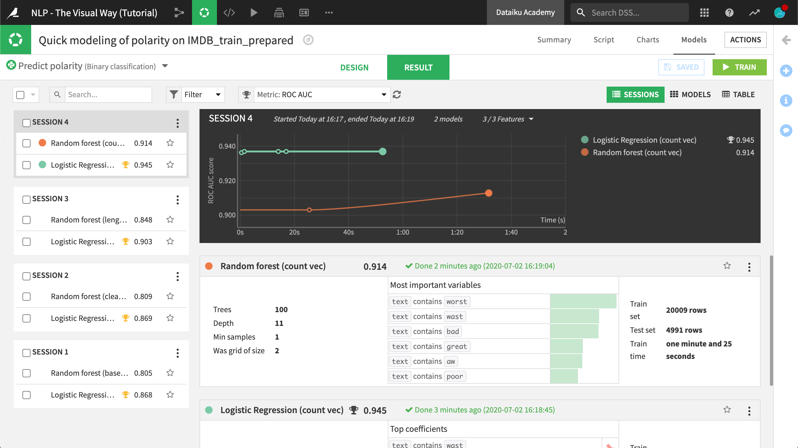
In addition to the performance boost, they also have an edge in interpretability. Whether looking at the most important variables for the random forest model or the top coefficients for the logistic regression model, we can see features like the text contains “bad”, “worst”, or “great”.

These benefits, however, did not come for free. While the training time for the “term hashing and SVD” models were all under 20 seconds, the count vectorization models took more than 1 minute. Depending on our use case, this could be a critical tradeoff.

On your own, try training more models with different settings in the Feature handling pane:

• Switch to “TF/IDF vectorization”.

• Observe the effects of increasing or decreasing the “Min. rows fraction %” or “Max. rows fraction %”.

• Include bigrams in the “Ngrams” setting by increasing the upper limit to 2 words.

Evaluate the Model

When you have sufficiently explored building models, the next step is to deploy one from the Lab to the Flow.

A number of factors– such as performance, interpretability, and scalability– could influence the decision of which model to deploy. Here, we’ll just choose our best performing model.

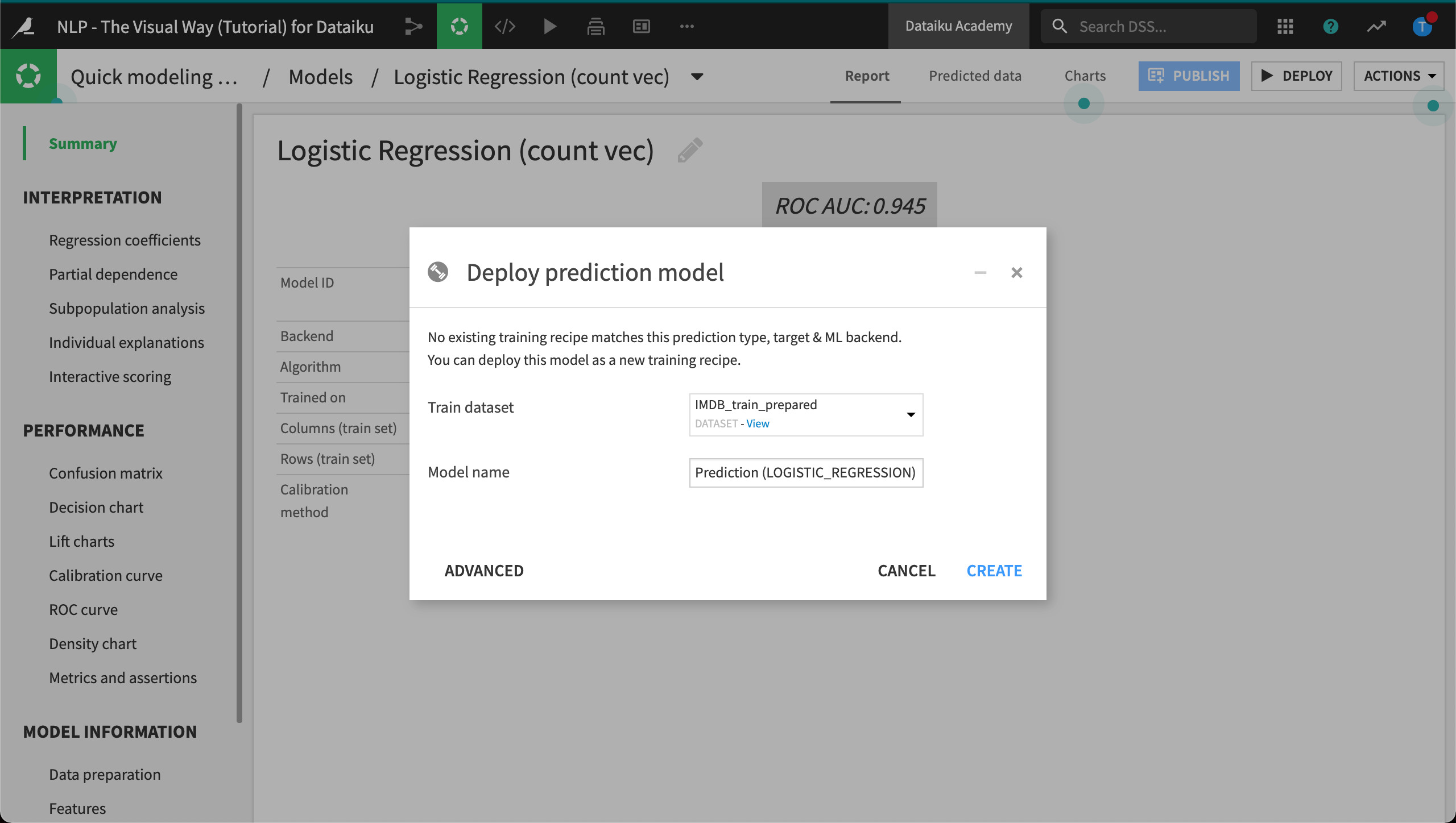
• From the Result tab of the modeling task, choose a model to deploy.

• Open the model summary.

• Click the Deploy button in the upper right corner.

• Click “Create”.

The relevant question is whether this model will perform as well on data that it has never faced before. A steep drop in performance could be a symptom of some level of overfitting the training data.

The Evaluate recipe can help answer this question. But first, we need to ensure that the test data passes through all of the same preparation steps that the training data received. We’ll start by copying the existing Prepare recipe.

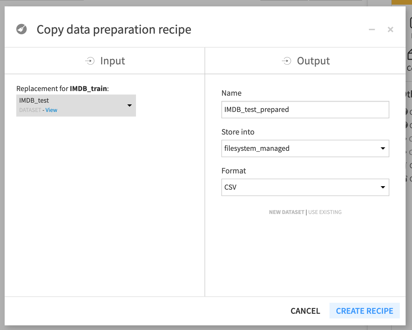
• Select the Prepare recipe (compute_IMDB_train_prepared).

• In the Actions sidebar, choose Copy.

• Change the input dataset to IMDB_test.

• Name the output dataset IMDB_test_prepared.

• Create and run the copied recipe containing the same preparation steps.

Warning

IMDB_test does not have a sample column. Accordingly, we need to adjust the copied Prepare recipe steps. Change the first step to remove only sentiment instead of sentiment and sample.

Once the test data has received the same preparation treatment, we are ready to test how the model will do on this new dataset.

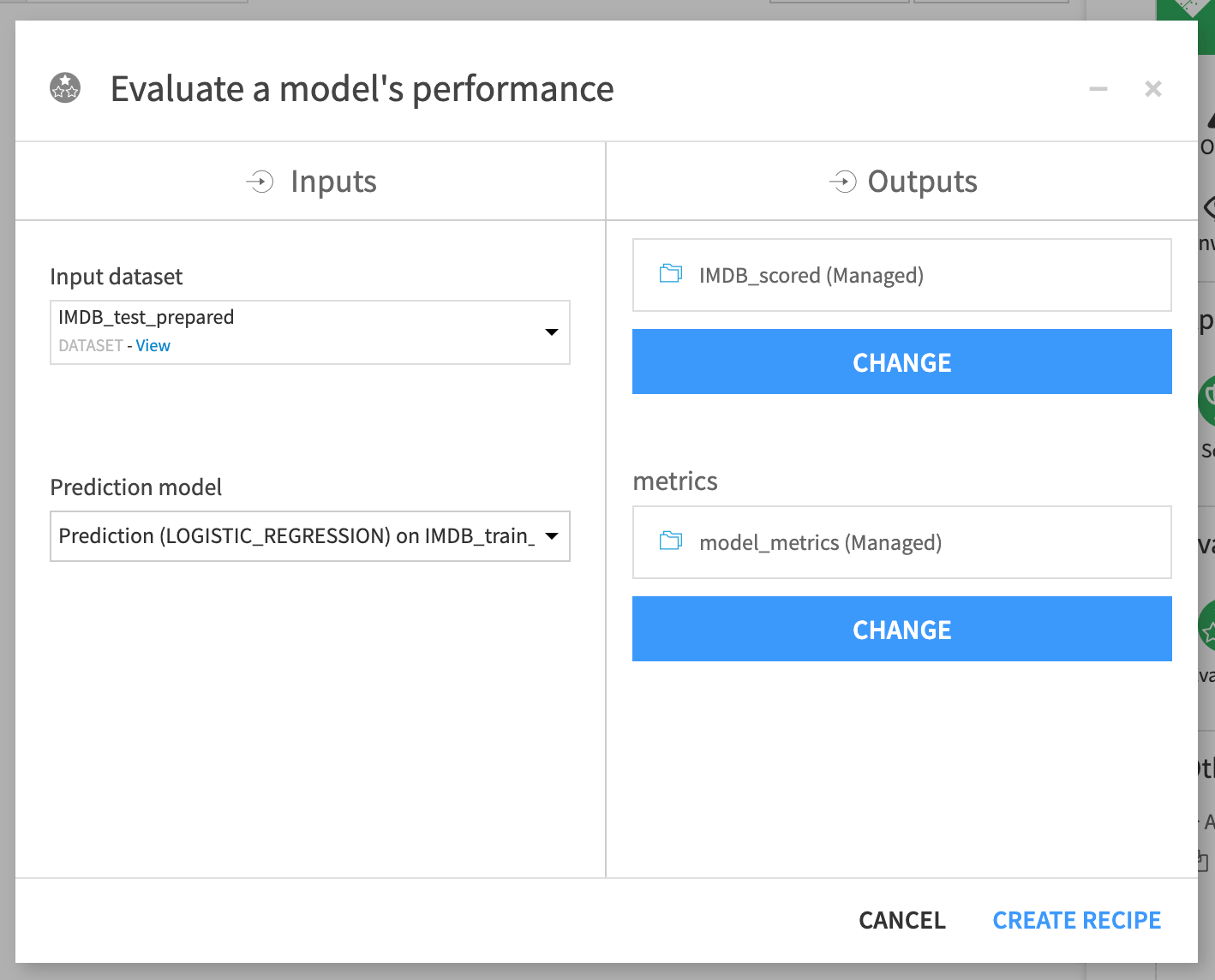
• From the Flow, select the deployed model and initiate an Evaluate recipe from the Actions sidebar.

• Choose IMDB_test_prepared as the input dataset.

• Name the output datasets IMDB_scored and model_metrics.

• Click “Create Recipe” and then run it.

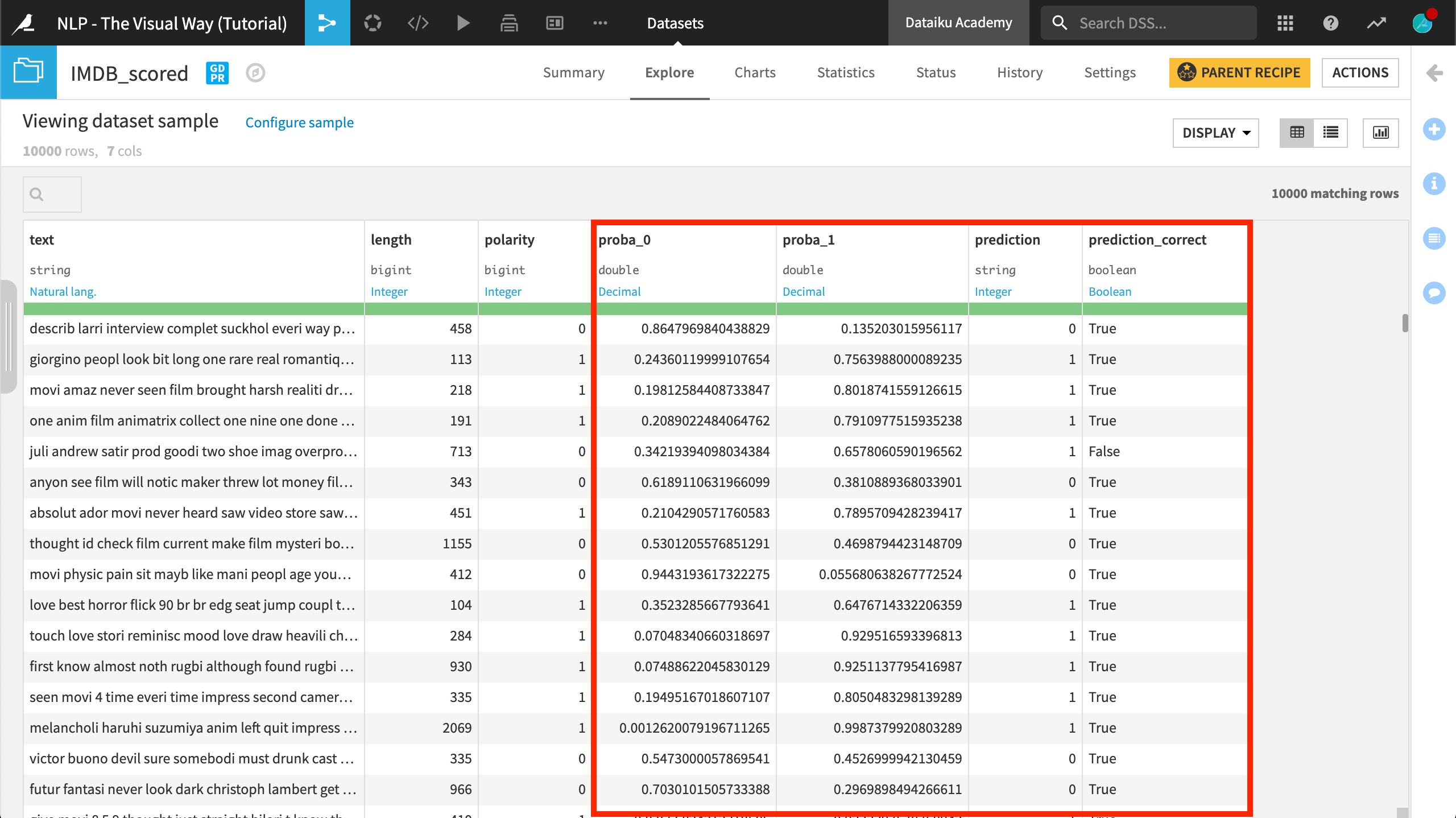
The Evaluate recipe produces two output datasets:

• The recipe has appended class probabilities and predictions to the IMDB_scored dataset.

• The model metrics dataset logs the performance of the active version of the model against the input dataset. Overall, it appears that the model’s performance on the test data was very similar to the performance on the training data.

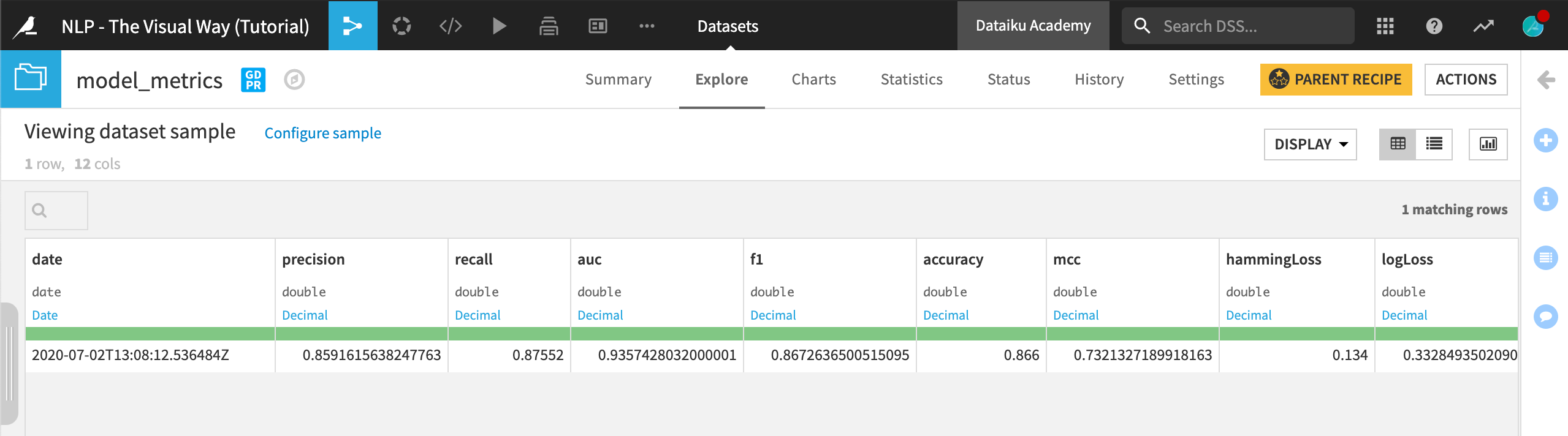
As we update the active version of the model, we could keep running the Evaluate recipe to check the performance against this test dataset.

What’s Next?

Congratulations! You have successfully built a model to perform a binary classification of the polarity of text. Along the way, you:

• learned the importance of text cleaning and feature engineering

• explored the tradeoffs between different text handling strategies, and

• evaluated model performance against a test dataset.

This was just the start of what you can achieve with Dataiku DSS and NLP! In another course, we’ll show more advanced methods using code.

Tip

For a bonus challenge, return to the sentiment column provided in the raw data and try to perform a multiclass classification. You’ll find that the distribution of sentiment is bimodal. No one writes reviews of movies for which they don’t have an opinion! Perhaps use a Formula to add a third category to polarity (0 for very low sentiment scores, 1 for middling, and 2 for very high). Are you able to achieve the same level of performance with the addition of a third class?