Integration with Amazon Redshift

Amazon Redshift is one of the analytical databases DSS can easily work with. This article shows how to integrate these 2 technologies.

Loading data into Redshift with DSS is as simple as:

• create your connection to Redshift and S3

• load your dataset into S3 with the proper format and in the same zone as your Redshift instance

• load your data from S3 to Redshift using a “Sync” operator

That’s it. DSS will take care of the plumbing for you and let you focus on analyzing your data.

The rest of the course provides a hands-on exercise.

Technical Requirements

We assume here that you have access to a Redshift instance (otherwise see the docs on how to create one from your Amazon AWS console), and that you have access to a S3 bucket with the proper “write” privileges.

Define the Redshift connection

Go to the Administration interface in DSS, and create a new “Redshift” connection:

Fill in your credentials as prompted:

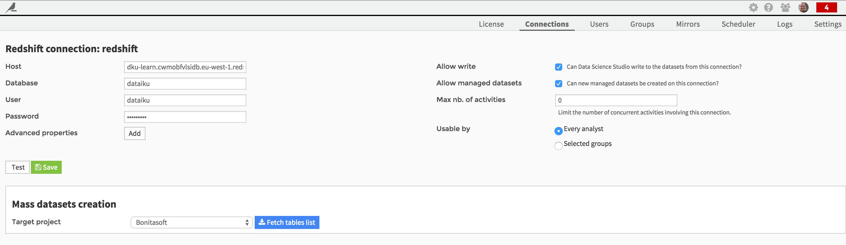
You’ll need to know a few pieces information, including the database’s password.

Define the S3 connection

From the Administration interface again, and create a new “Amazon AWS (S3)” connection:

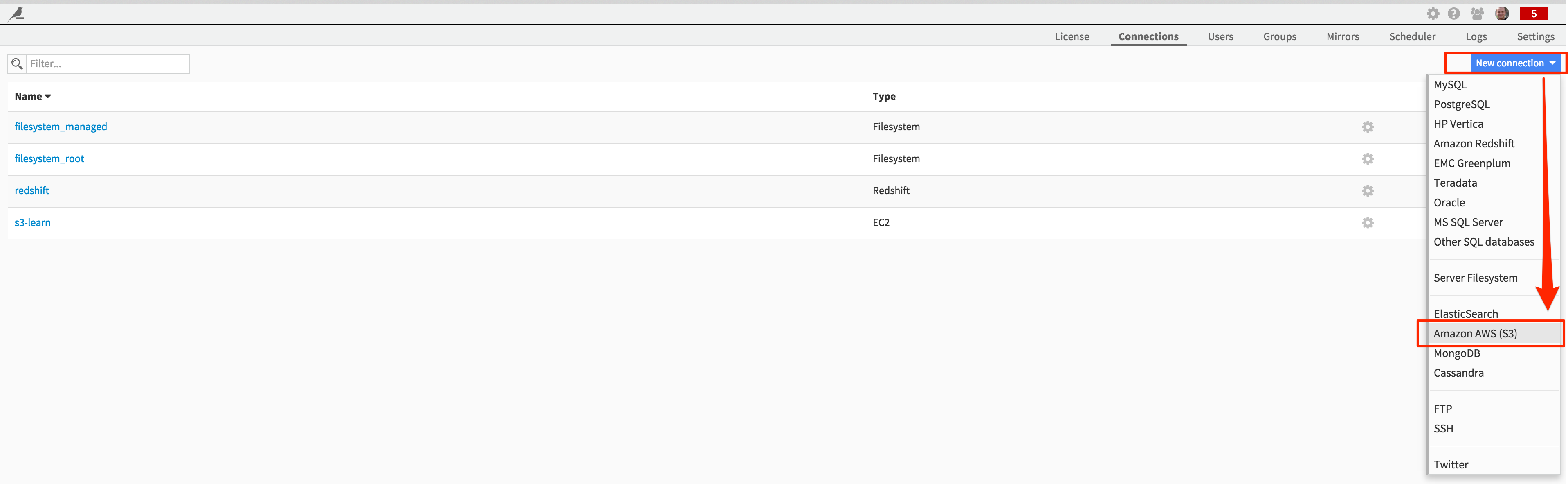
Fill in your credentials as prompted:

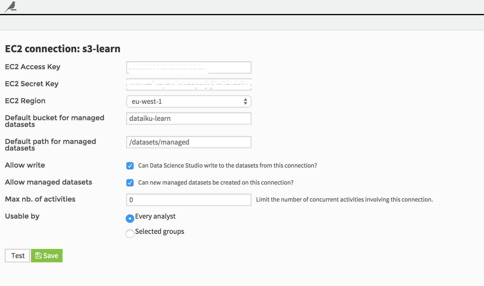
Please note that you’ll need to know a few pieces of information, including your Amazon credentials, and a bucket where you can read and write data.

Get some (big) data

In this example, we are going to use Github data. Specifically, we’ll use data from the GitHub Archive, which is a project to record the public GitHub timeline, archive it, and make it easily accessible for further analysis. These data are very interesting since they provide very detailed and granular events, letting us looking for interesting insights from open source software projects.

We have access here to 6 months of Github activity history (from January to June 2015), stored on our server as JSON files split by hour (one hour == one JSON file).

As usual, the first step is to create a DSS Dataset on top of these files:

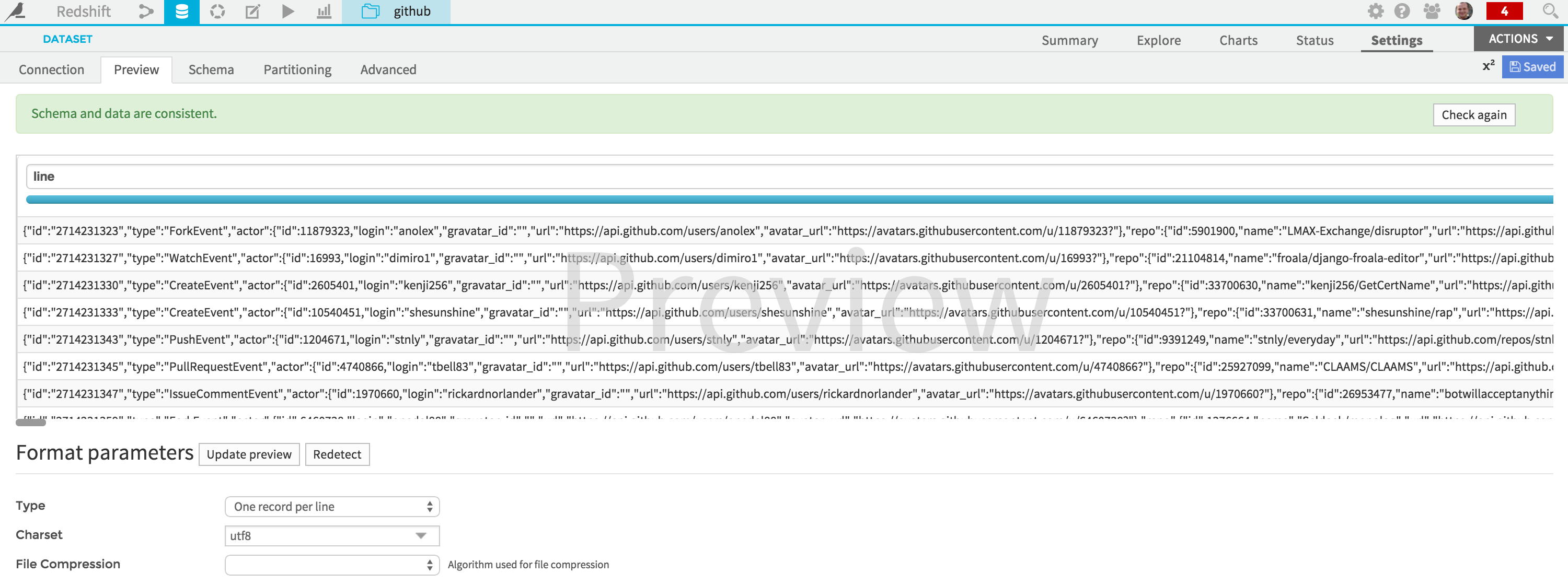
Please note that the selected format is “One record per line”, since we do not want to flatten the JSON file yet due to its very rich nature.

Also, we define a partitioning scheme, allowing us to efficiently work on daily subsets of data:

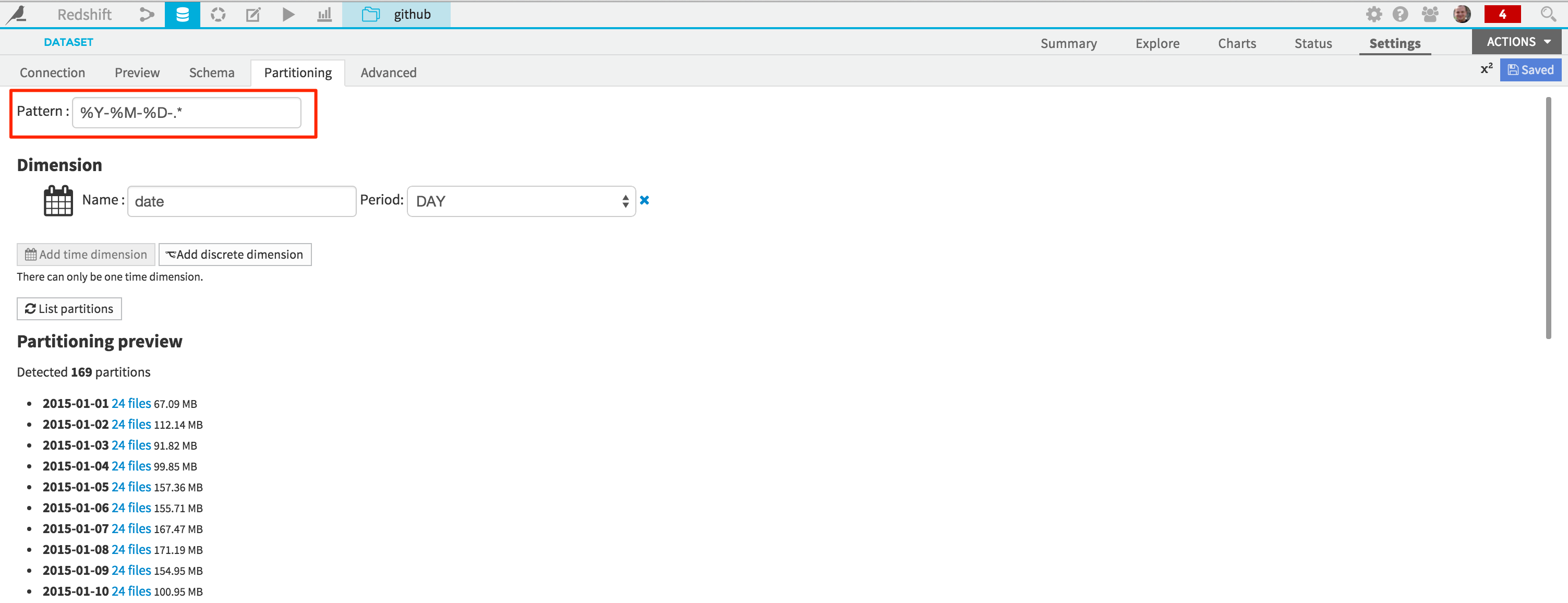
You can now save the input dataset (named “github” here):

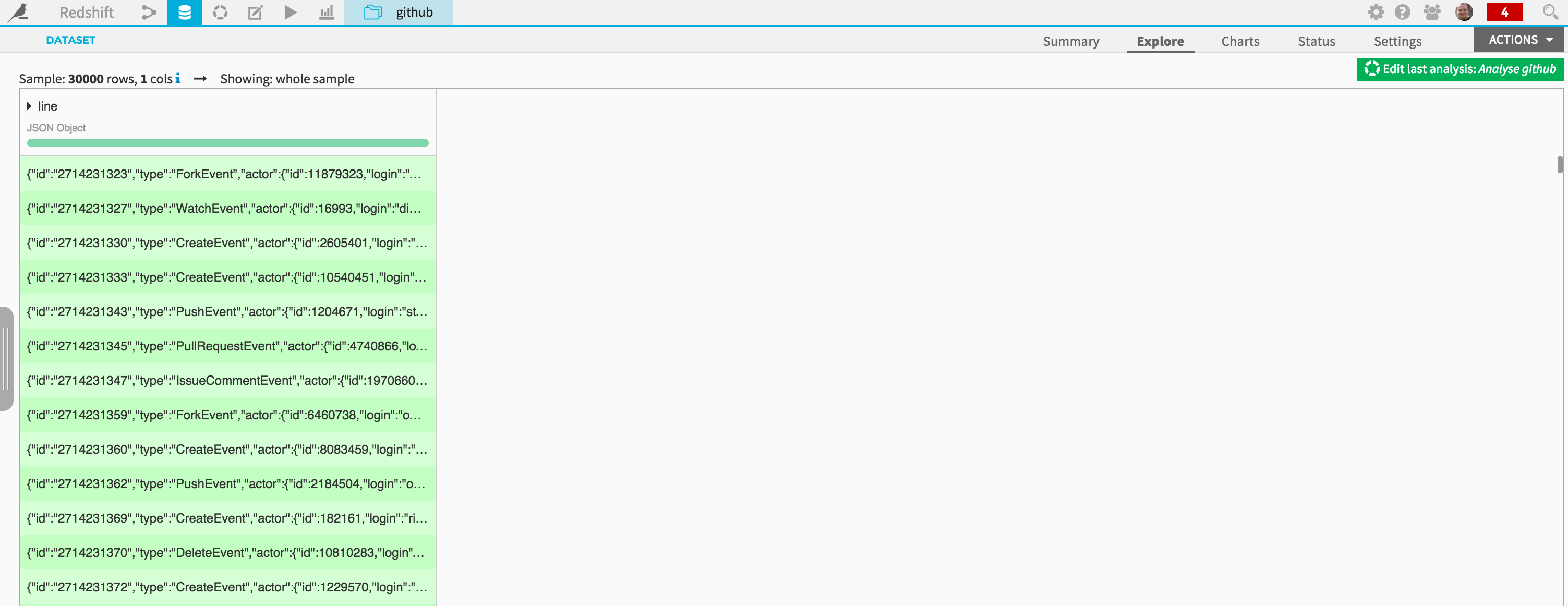
Note that you see here the raw JSON content, with one event per line, stored in a fairly large 30Gb dataset (compressed) with 90 millions records for this 6 months period. Also, the column has automatically be named “line”.

Push your data to S3

Loading data effectively into Redshift requires the files to be available on S3, along with a few other constraints well documented here.

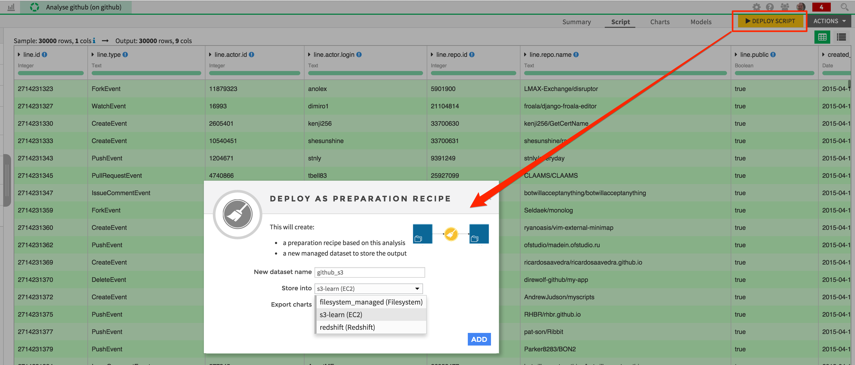
For the sake of simplicity, we will not use all the information available in the initial dataset. To create a new dataset with a suitable (tabular) format for Redshift, create a new Analyze script on the initial dataset.

As we are only interested, for now, in looking at the global activity and popularity of the Github repos, the visual data preparation script we build does the following:

• flatten the JSON structure (not going beyond 1 level depth)

• flatten the “actor” and “repo” sections of the JSON

• create a new “date” column that will be used for Redshift partitions

• remove the unnecessary columns

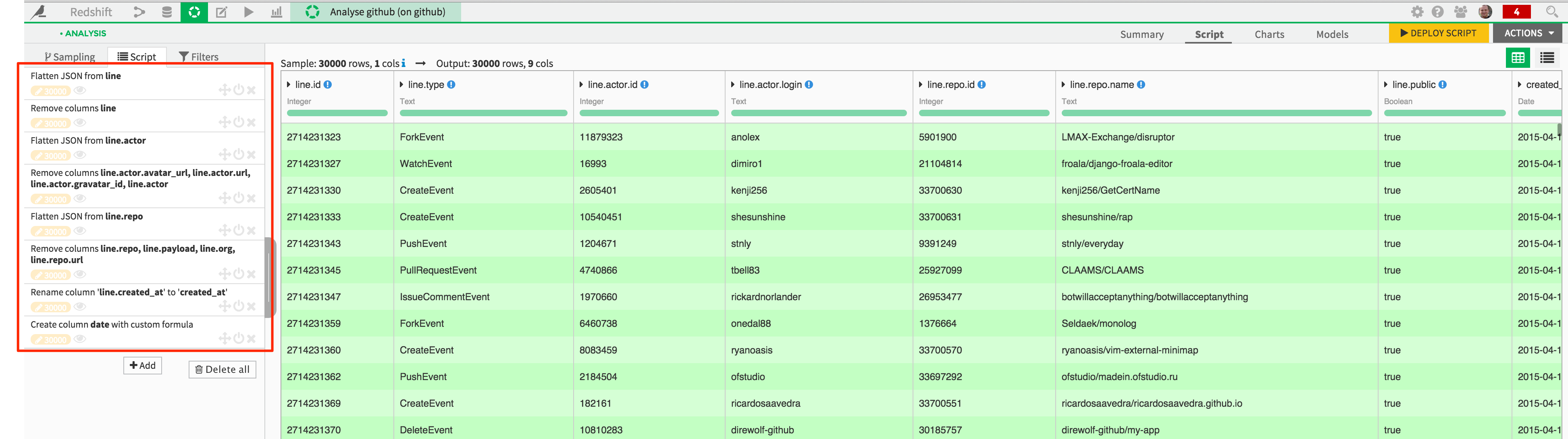
This script can now be deployed, and the resulting dataset written on Amazon S3. Click on the “Deploy Script” button, and store the newly created “github_s3” dataset in your S3 connection.

A new recipe has been created, with the local “github” dataset as input, and the “github_s3” dataset as output. Note that the daily partitionning scheme of the input dataset has automatically been copied to the output.

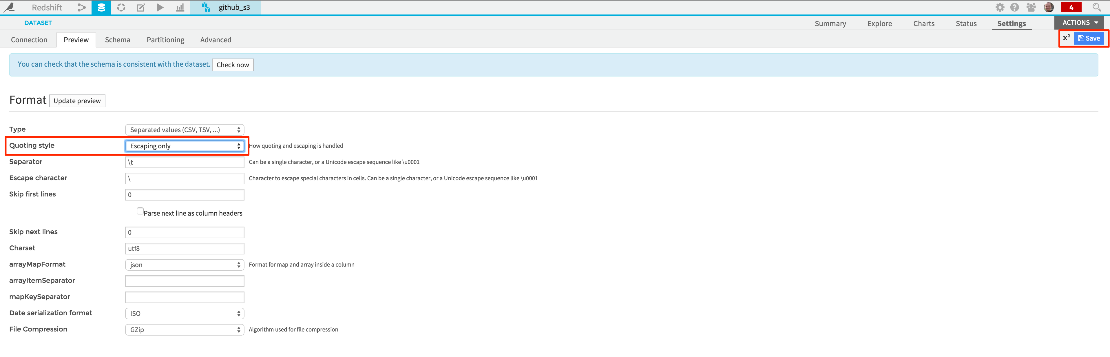
Before actually building your dataset (i.e putting your data on S3), and to comply with the Redshift constraints, click on the link to the new “github_s3” dataset, and go to the “Settings” tab. Change the quoting style to “Escaping only”, and save your changes.

Go back to the Flow screen (click on the button in the nav bar or hit “g + f” on your keyboard), and click on the “github_s3” dataset icon. In the right panel, click on “Build”, and load a few days to begin, the month of January 2015 for instance:

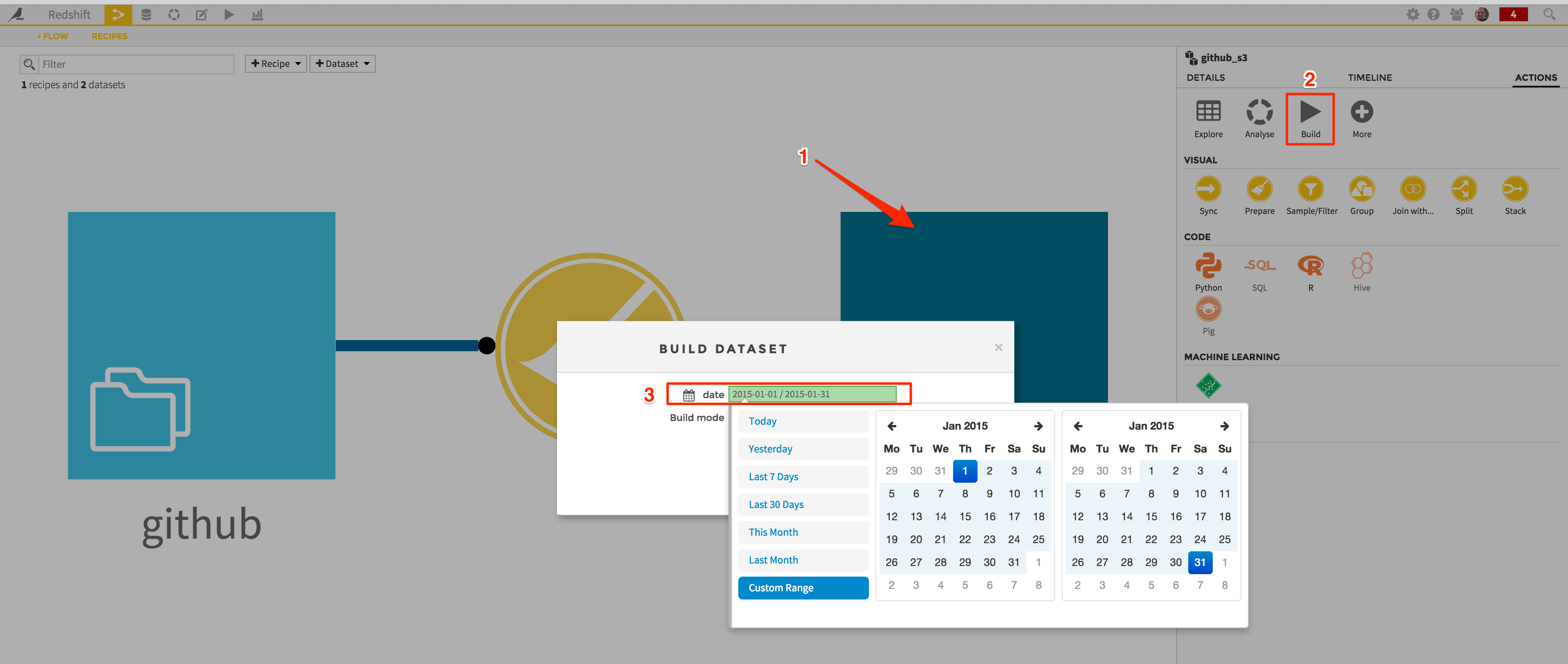
Once everything set, hit the “Build” button. A new job is launched, that will:

• start from the input files

• apply the visual data preparation script

• load it into S3 with the proper format on the fly.

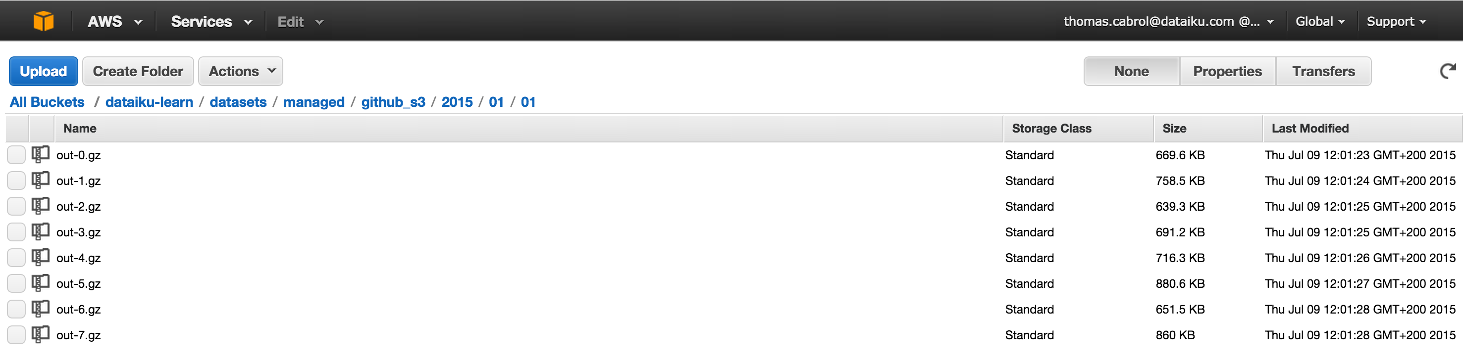
With our servers, it takes approximatively 2 minutes to load a month worth of data:

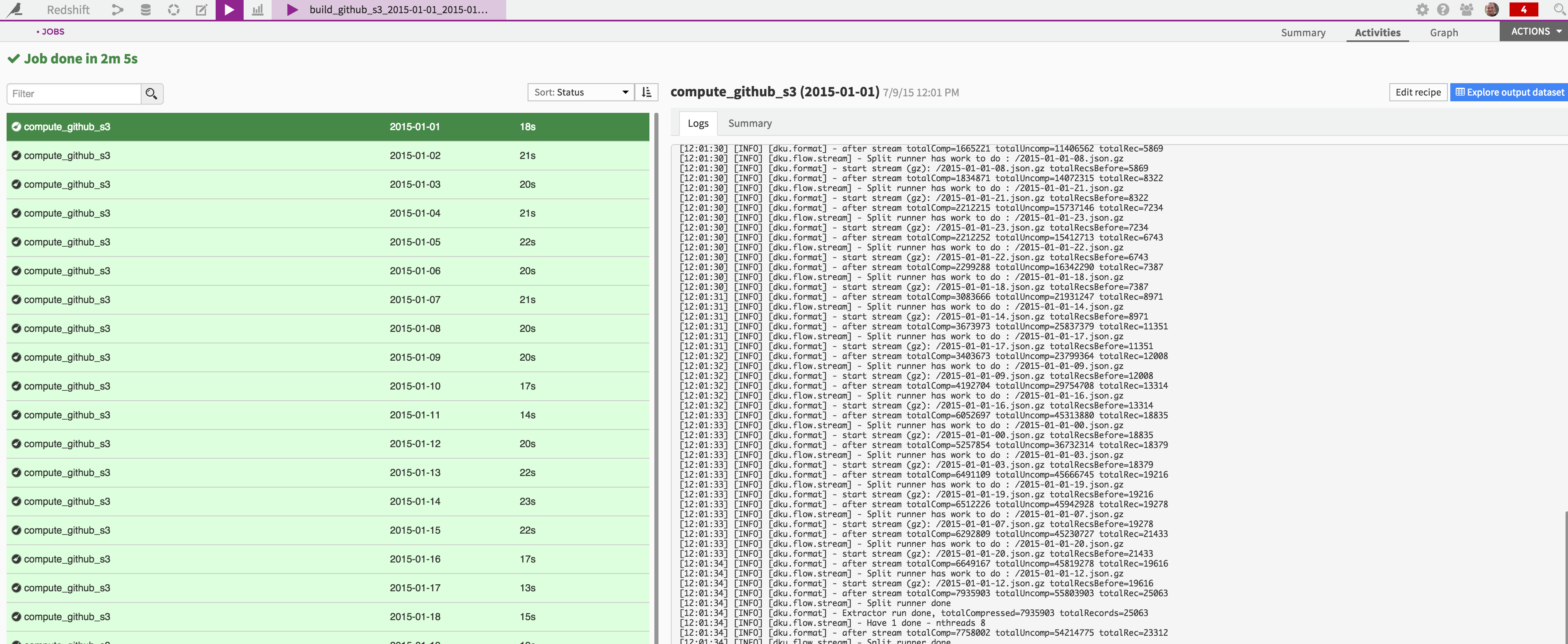
That’s it, your data sits now in S3 and is ready to be loaded in Redshift:

Load your data to Redshift

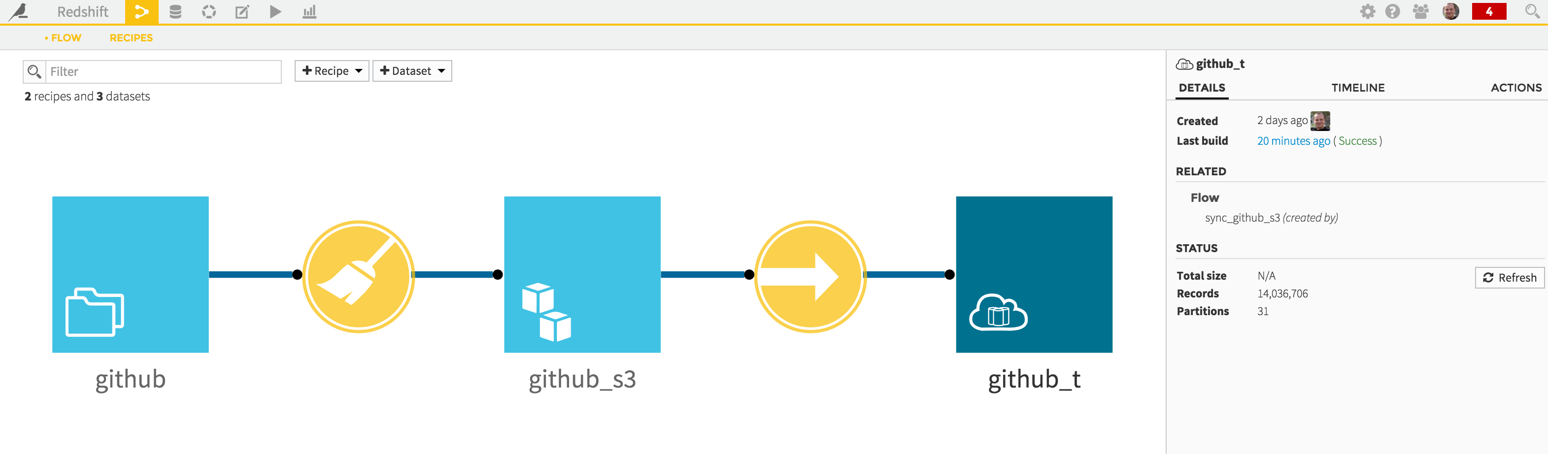
Loading your dataset into Redshift will now be very easy. Just go back to the Flow screen again, and create a new “Sync” recipe from the “github_s3” dataset:

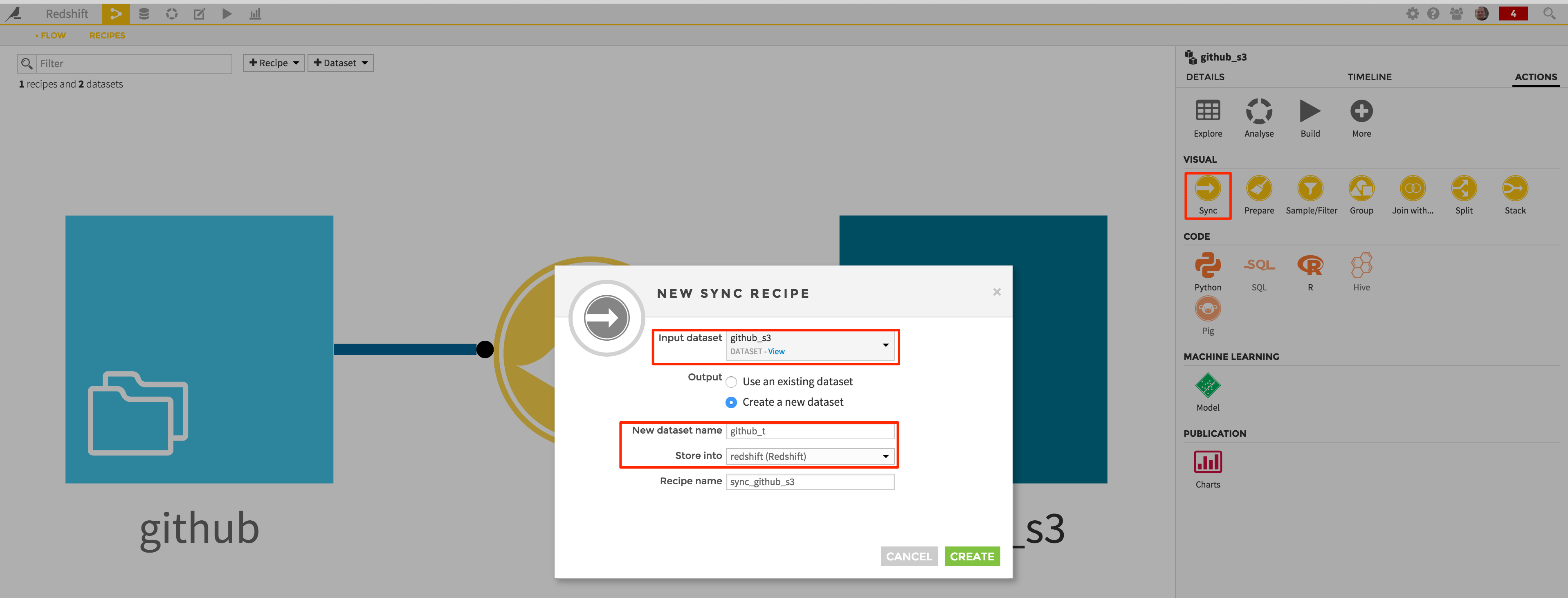
This will create a new “github_t” dataset, stored in your Redshift connection.

The summary screen showing up will let you see again the input / output of your Sync recipe (note that again the partitioning scheme is copied), and build (i.e copy your S3 data to Redshift) your dataset directly from there:

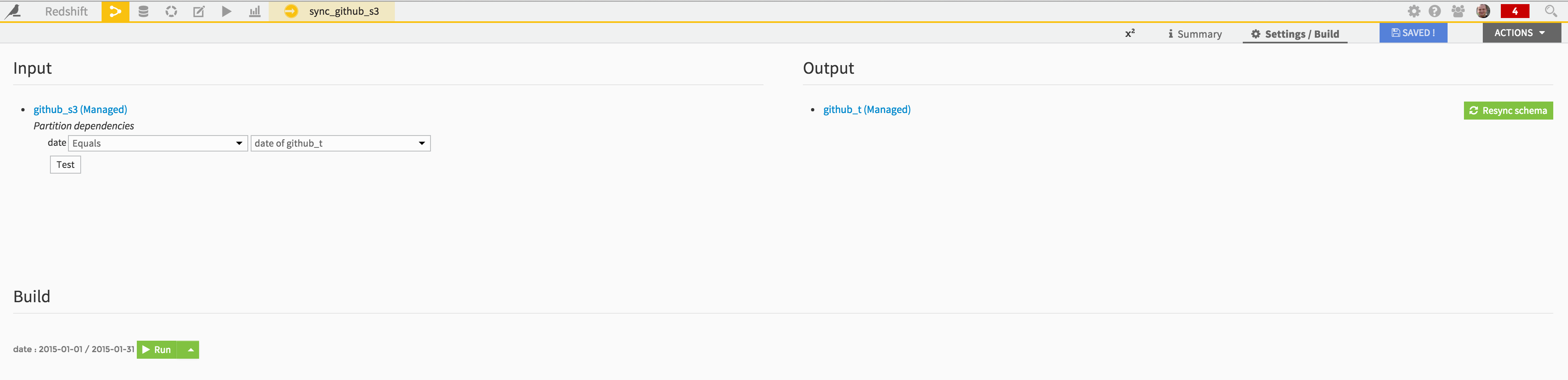
Hit the “Run” button and wait for the job to complete:

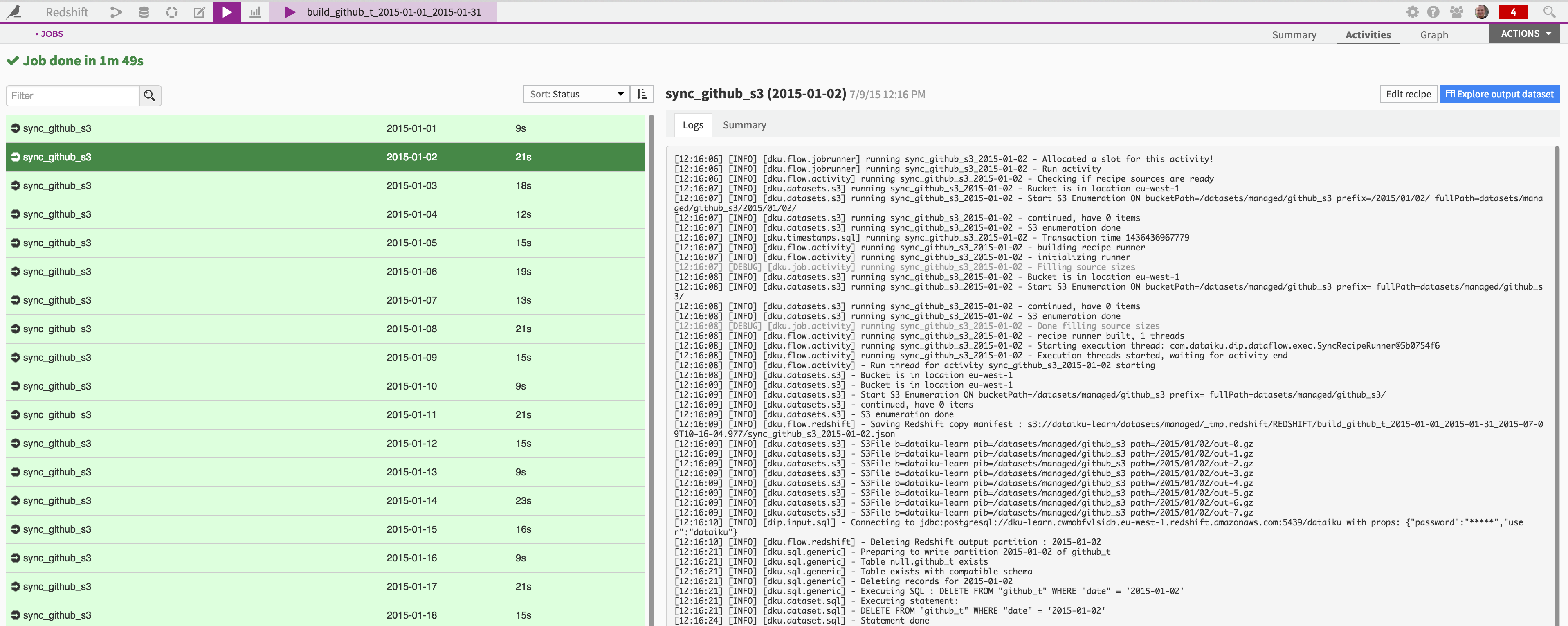
A little bit less than 2 minutes to wait, and your data is in Redshift! And note that the resulting table is partitioned, and we didn’t even have to care about its schema.

What’s Next

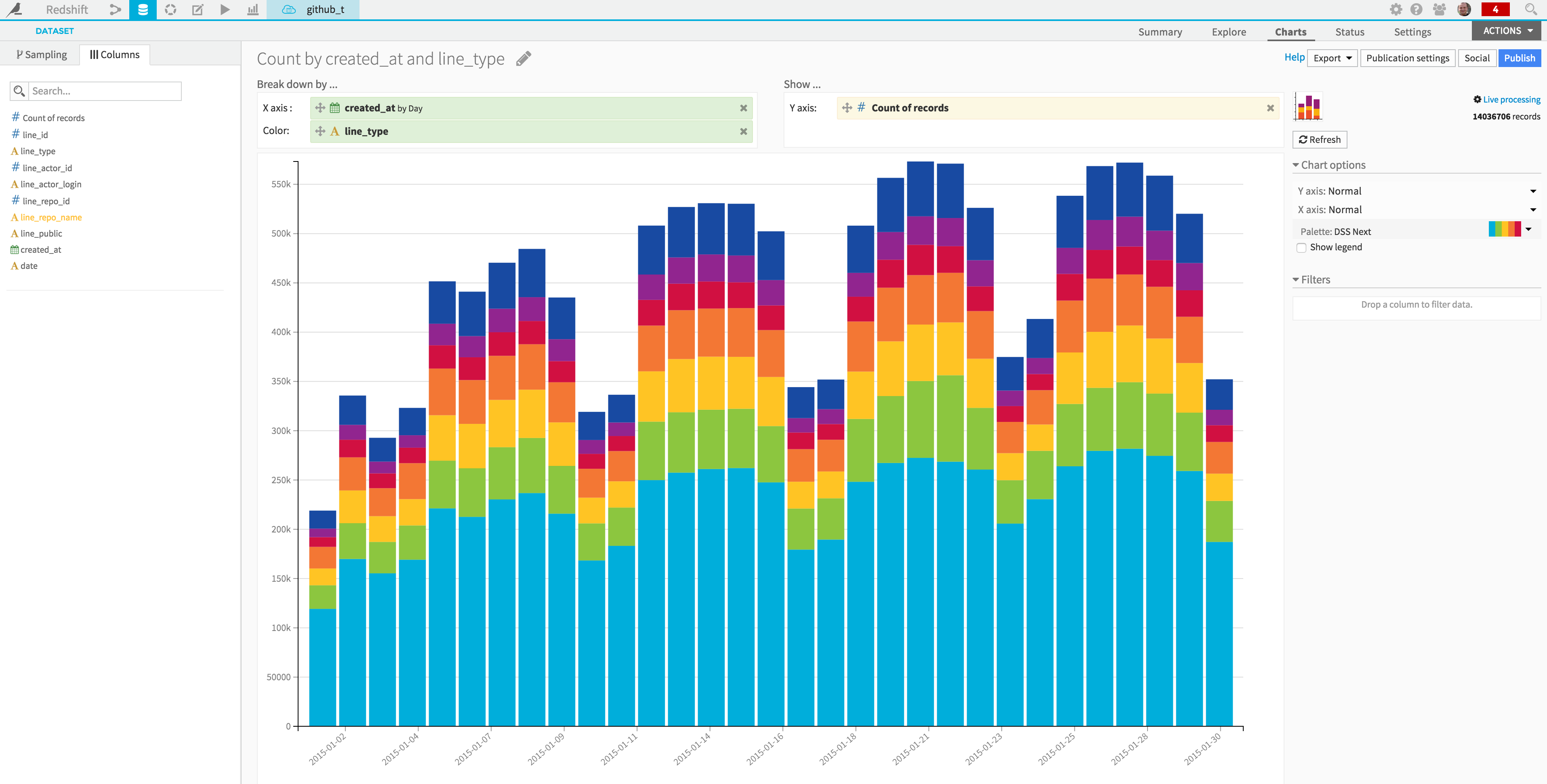
You can for instance easily create Charts on the Redshift dataset. Because Redshift can be used interactively thanks to its performance, Charts can be switched to “Live processing” (i.e Redshift will do most of the aggregation work):

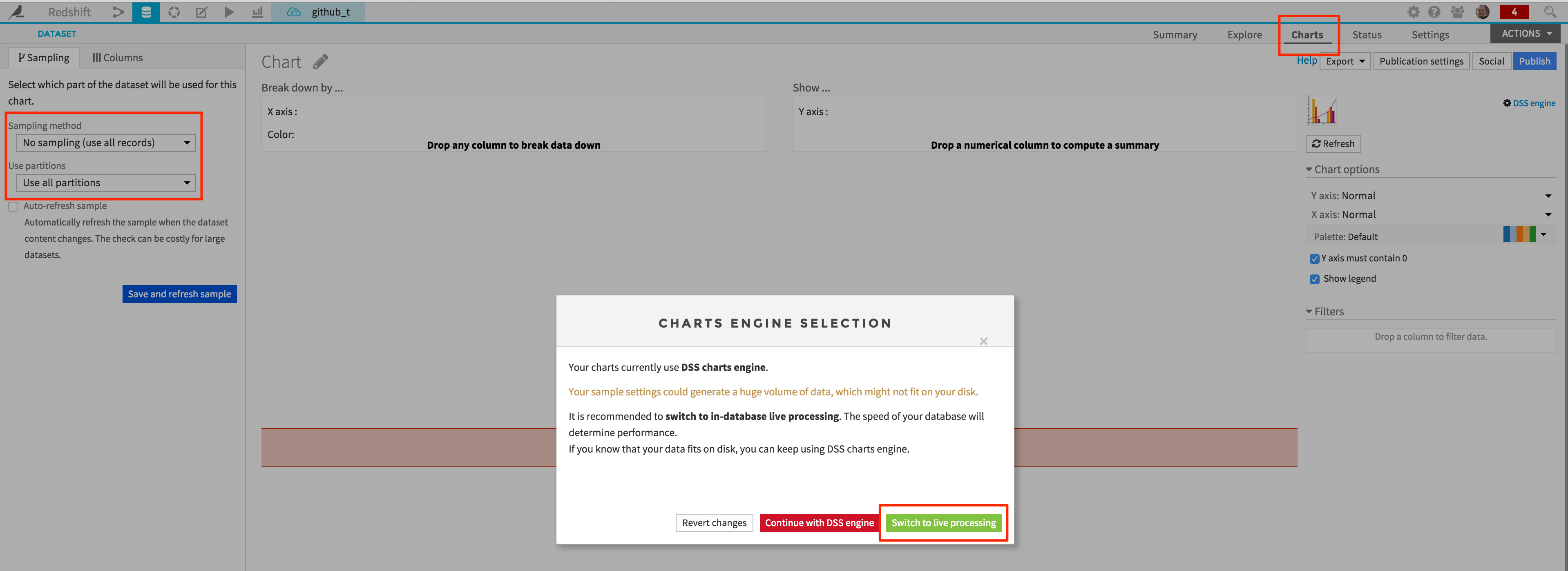
Because live processing is enabled, Charts will be based on the entire dataset:

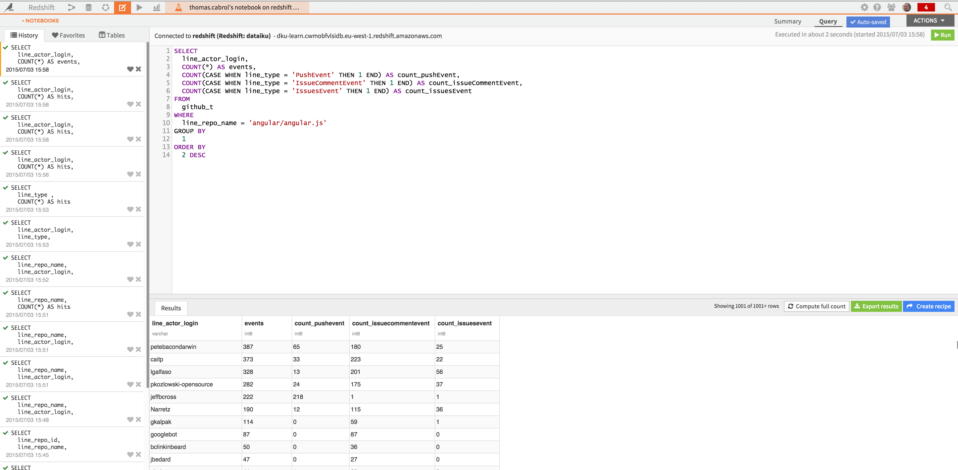
You may also want to analyze interactively the dataset with your own SQL queries, using a SQL notebook:

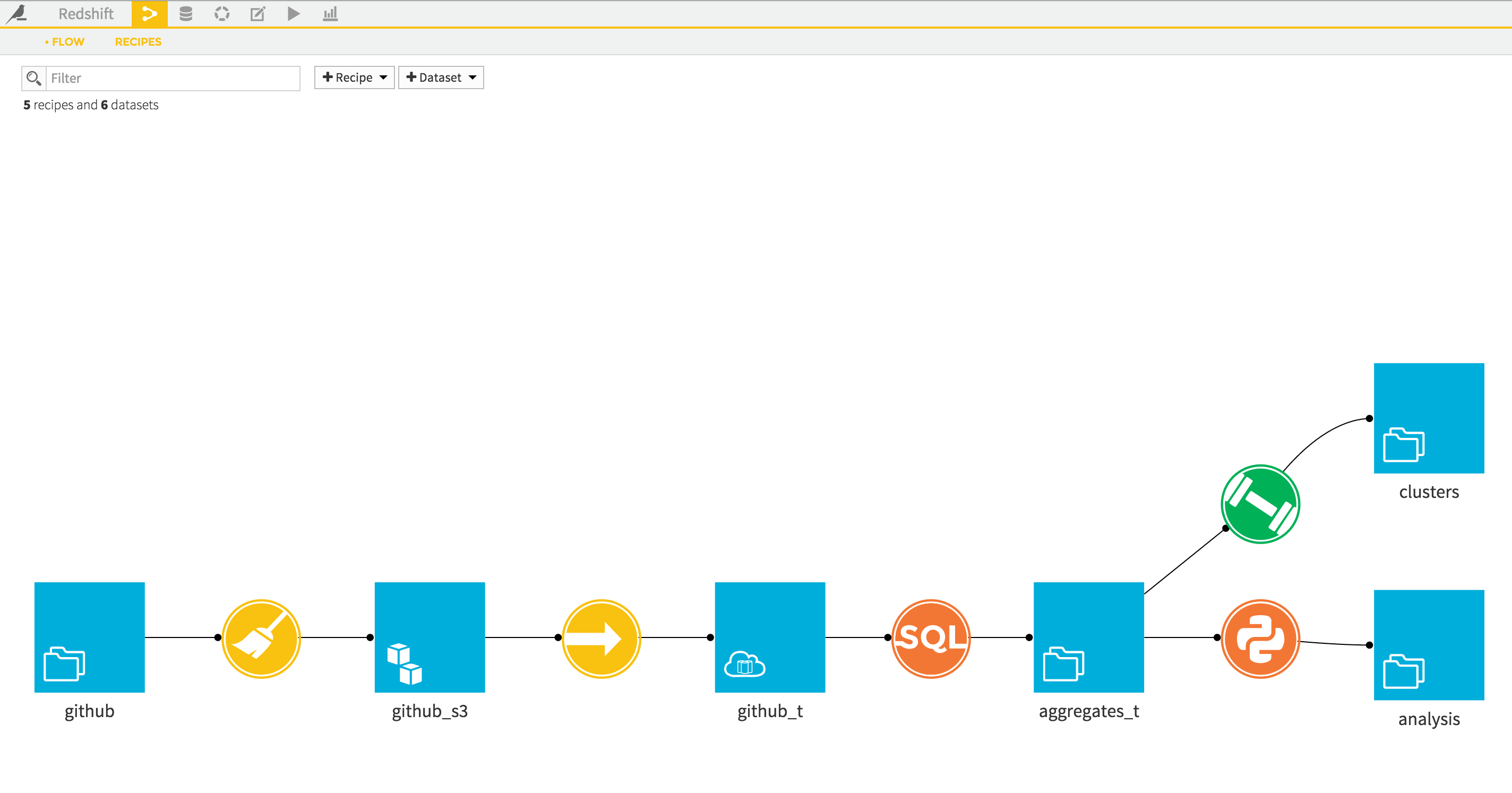
And finally, you could also write a SQL recipe in a larger workflow, for instance if you were to use Redshift to aggregate and reduce the size the base data, before passing it to R or Python for deeper analysis, or create a Model from it:

We’re done. A few steps will take your data into Redshift, and you’ll be good for large scale analysis in a matter of minutes.