Concept Summary: Regression Algorithms

Regression is a supervised learning technique for determining the relationship between a dependent variable, y, and one or more independent variables, x. Two common regression algorithms are simple and multiple linear regression.

Simple Linear Regression

We’ll use a simple linear regression algorithm to predict a student’s exam score, given how long the student studies. This is a regression problem because we’re predicting a continuous quantity, rather than a class label, as we would in a classification problem.

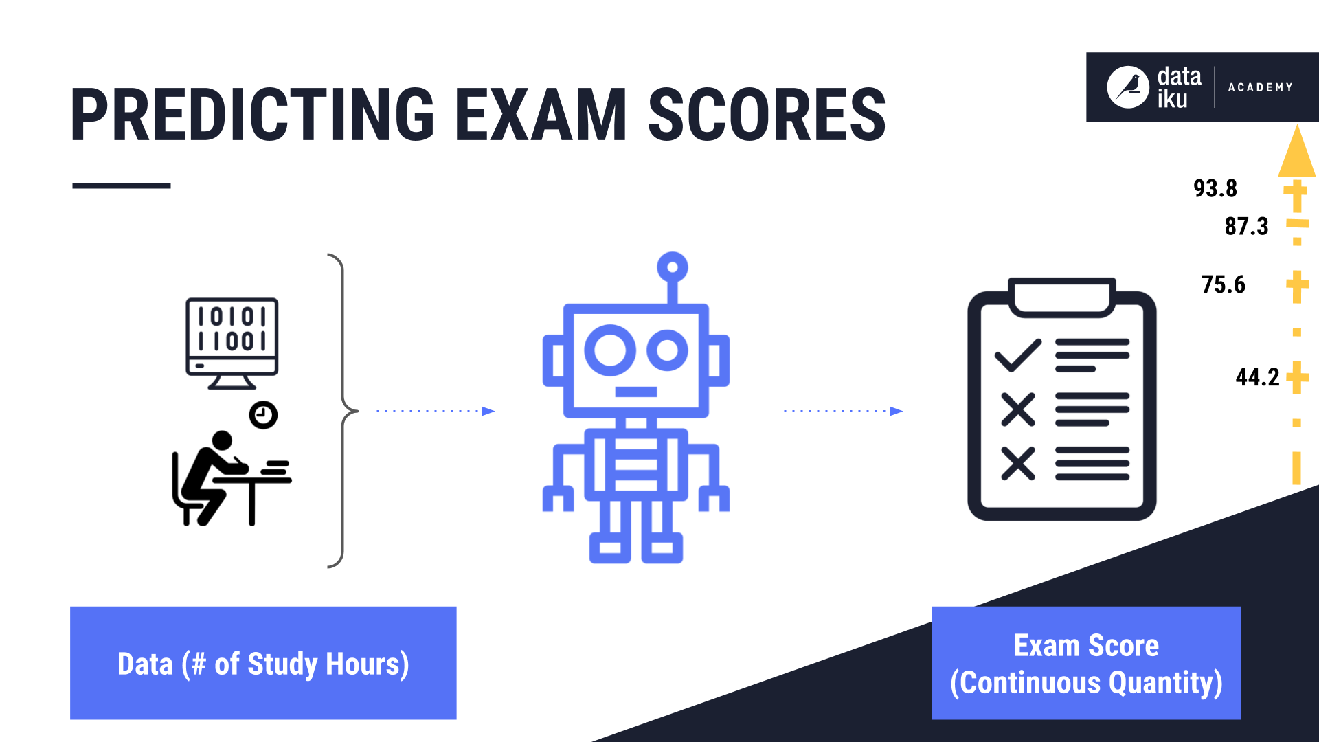
Our independent variable is the number of sleep hours. When plotting student exam scores based on hours of study, linear regression plots a line that best fits the data points. It does this by applying the formula, “y = b0 + b1* x”, where:

• y is the exam score,

• x is the number of study hours,

• b0 is the point where the line crosses the exam scores axis, also known as the y-intercept, and

• b1 is the change in the score based on the slope of the regression line

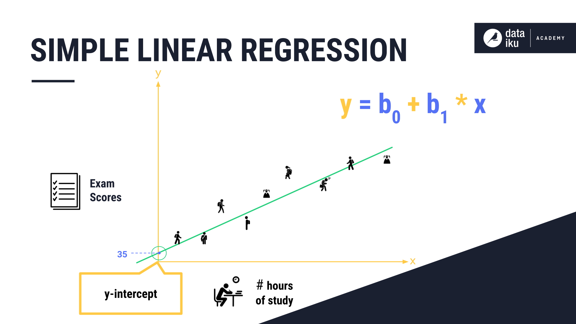
Note that 35 is the starting point of the score. In our example, students with zero study hours, will still achieve a minimum score of 35, taking into account credit for things like attendance and mid-year assignments.

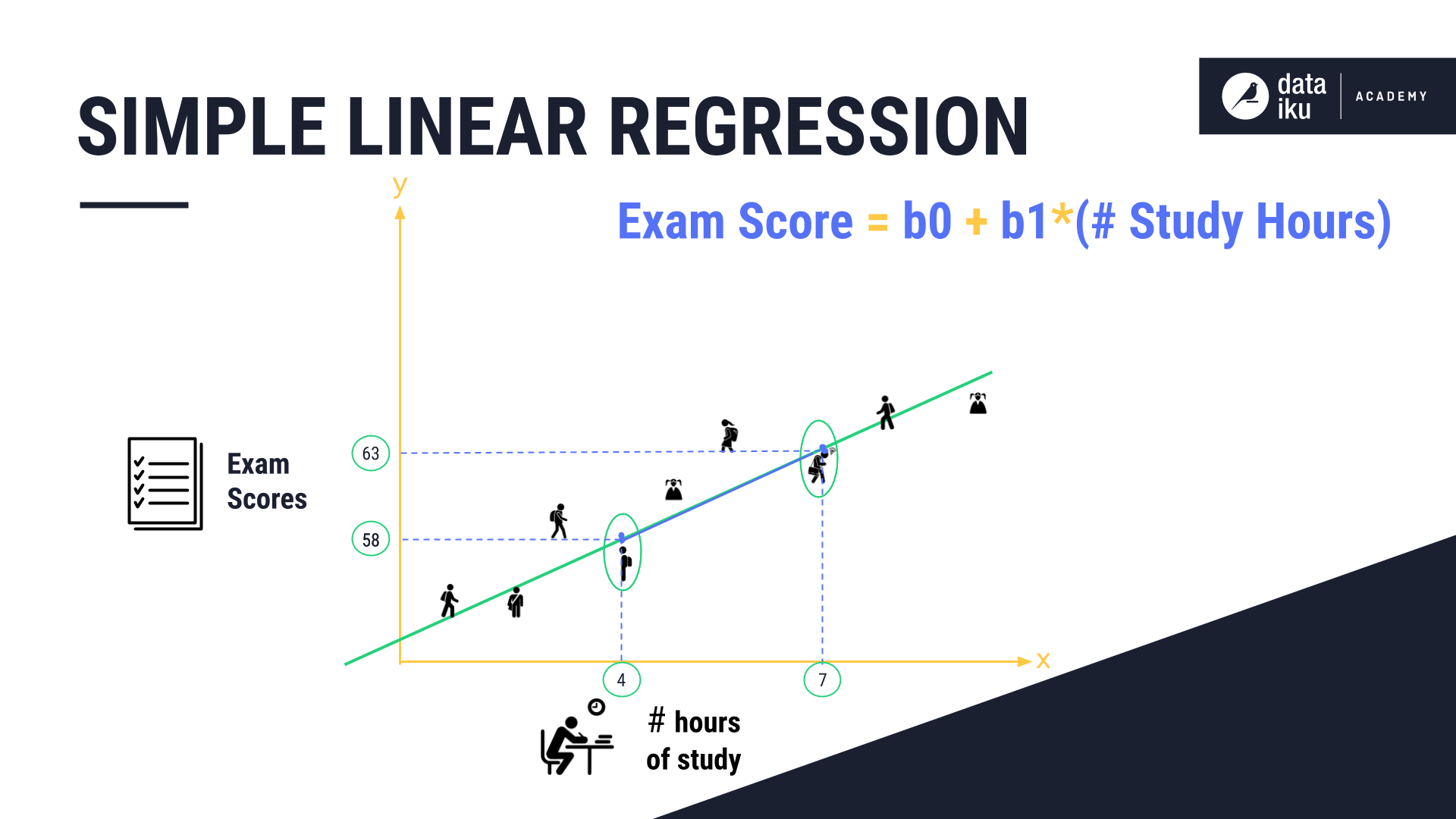
In our example, the difference between four and seven hours of studying increased the exam score by five. The equation of the exam score is equal to b0 + b1* (Number of Study Hours). The linear regression algorithm can then provide predictions by plotting the historical data.

In linear regression, the values that multiply the predictor values are known as coefficients–the mean change in the predicted response given a one unit change in the predictor.

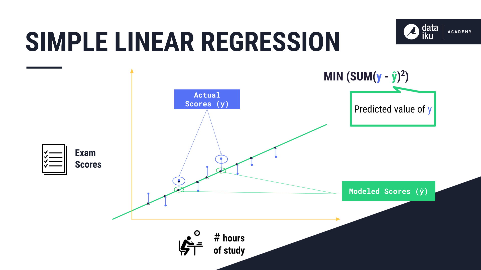
Let’s examine the vertical lines drawn from each data point to the linear regression model, where the equation MIN (SUM(y - ŷ)2) provides the best fitting line, y is the dependent variable, and ŷ is the predicted value of y.

To find the best fitting line, we first calculate the difference between the actual scores y, and the modeled scores on the regression line ŷ. We then square these differences, sum them up, and find the line that minimizes the sum of the squared differences as the best fit line. This line can then be used to predict the score of a new data point.

Multiple Linear Regression

In multiple linear regression, the value of the target variable changes based on the value of more than one independent variable, or x. In our example, the predictors are the number of study hours, and the number of sleep hours.

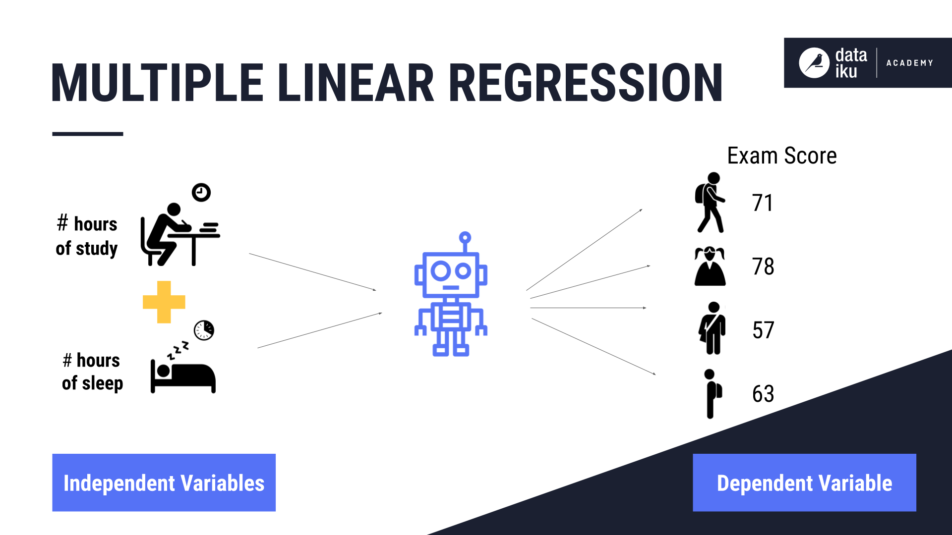
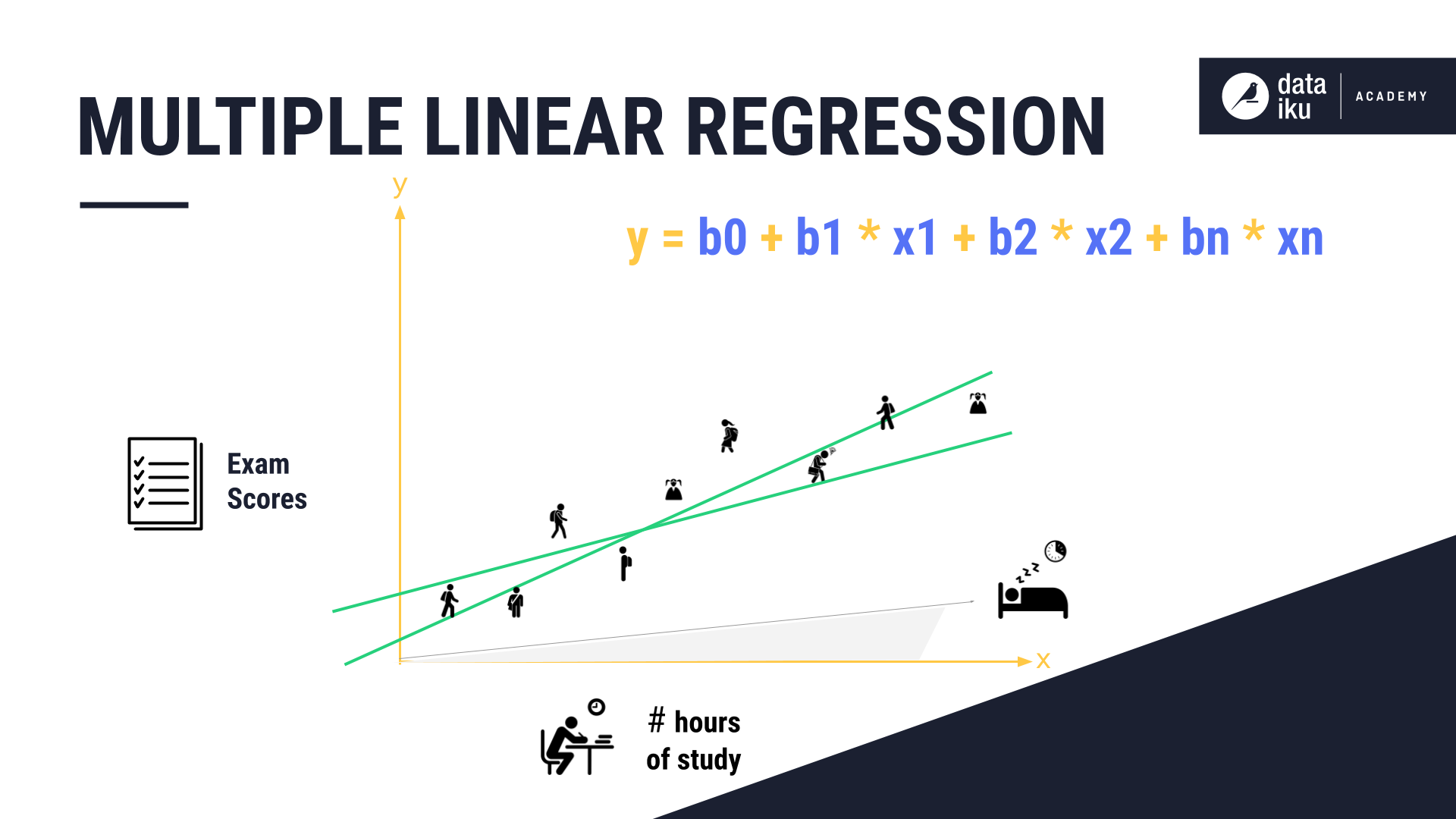
When plotting these two variables, the formula used by the algorithm is:

\[\]

y = b0 + b1 * x1 + b2 * x2 + bn * xn

And so on, for the number of independent variables used as inputs.

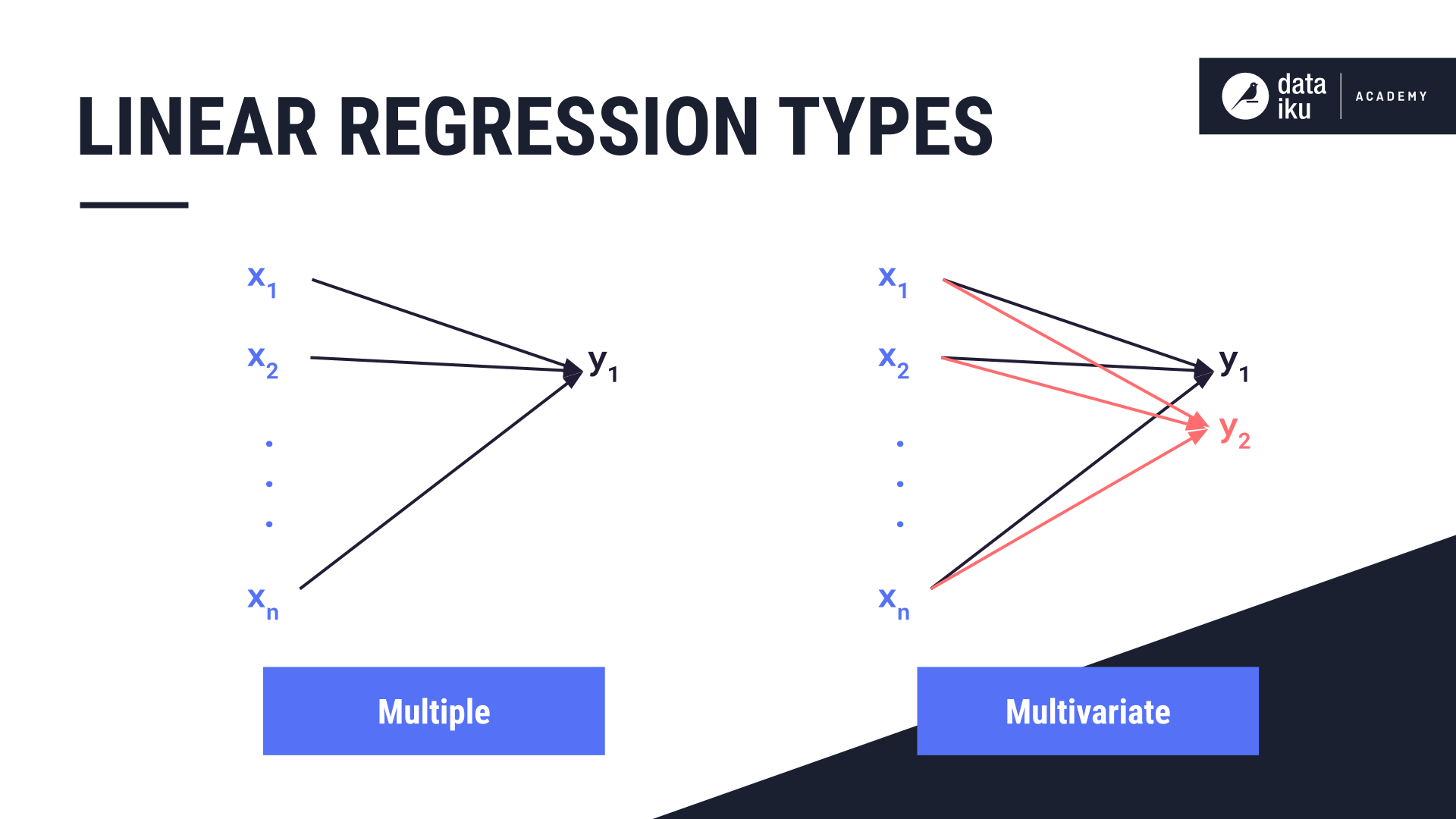
Multiple linear regression is sometimes confused with multivariate regression, which has more than one dependent variable, or y.

What’s next

In the Classification section, we will learn about logistic regression, which is a classification problem where we predict a categorical outcome rather than a continuous outcome.