Web Logs Analysis

Overview

Business Case

The customer team at Dataiku is interested in using the website logs to perform two kinds of analysis:

• Referrer Analysis

  • determine how visitors get to our website

  • identify who are the top referrers, both in terms of volume (number of visitors) and depth (number of pages linked)

• Visitor Analysis

  • segment visitors according to how they engage with the website

  • map these segments to known customers in order to feed them into the right channels (Marketing, Prospective Sales, and Sales)

Supporting Data

This use case is based on two input data sources. The downloadable archives are found below:

• Web Logs: The Dataiku website logs, spanning 2 months, that contain information about each individual pageview on the website.

• CRM: A simulated Customer Relationship Management (CRM) database containing transactional and demographic data about our clients.

Workflow Overview

The final Dataiku DSS workflow should look like the image below. You can also follow along with the completed project in the Dataiku gallery.

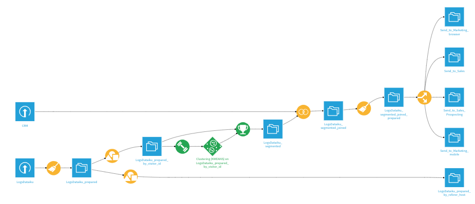
You will go through the following high-level steps:

• Upload the datasets

• Clean up and enrich the log data

• Use visual grouping recipes

• Run a clustering model to build segments

• Join the CRM and segment data for known visitors

• Customize and split dataset by segments

Prerequisites

You should be familiar with:

• The Basics courses

• Machine learning in Dataiku DSS

Technical Requirements

• The Reverse Geocoding / Admin maps plugin is required to produce administrative maps.

Create the Project

Create a new Dataiku DSS project and name it Web Logs Analytics.

Preparing the Web Logs Data

Create a new UploadedFiles dataset from the web logs data (LogsDataiku.csv.gz) and name it LogsDataiku.

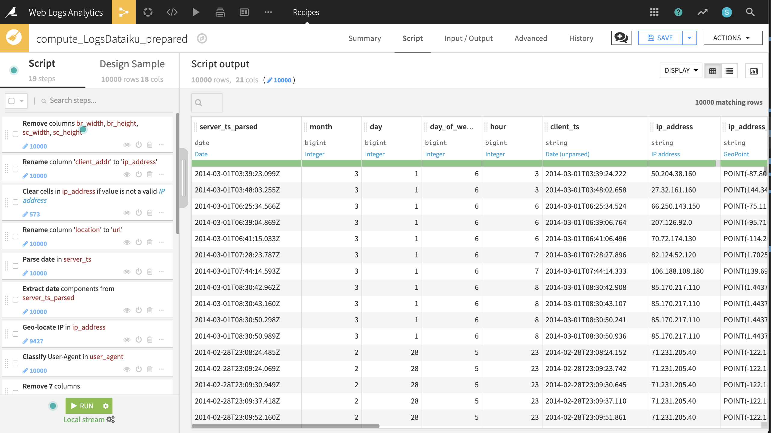
The dataset is already quite clean so the data preparation steps will focus mostly on enrichment and feature engineering. Create a Prepare recipe with LogsDataiku as the input and add the following steps to the script.

Hint

Clicking the down arrow to the right of the column header brings quick access to the most common data preparation steps for the column’s associated meaning. Many of the required steps below can be executed from this window.

• Cleaning

  • Remove four columns: br_width, br_height, sc_width and sc_height

  • Rename the column client_addr to ip_address

  • Clear invalid cells in the ip_address column for the IP address meaning

  • Rename the column location to url

• Feature engineering dates, locations, and user agents

  • Parse the server_ts column into a new Date column, server_ts_parsed, with format “yyyy-MM-dd’T’HH:mm:ss.SSS”

  • Extract four date components from server_ts_parsed: named month, day, day_of_week, and hour

  • Geo-locate the ip_address column, extracting the country, city and GeoPoint with the ip_address_ prefix

  • Classify, or enrich, the user_agent column

  • Remove user_agent and all of the enriched columns, with the exception of user_agent_type

Note

Note that parsing a date into the existing column will change the column’s meaning, but not its storage type. Parsing a date into a new column, on the other hand, changes both type and meaning. This will have consequences if you wish to perform mathematical operations on the column. For a more detailed guide on managing dates, please see the reference documentation.

• Feature engineering the Dataiku URLs

  • Split URL in url, extracting only the path

  • Split url_path on / and select Truncate so that it keeps only the first output column starting from the beginning

  • Fill empty cells of url_path_0 with home using the “Fill empty cells with fixed value” processor

  • Create dummy columns from values of url_path_0 using the Unfold processor. This step creates new columns representing the section of the website the visitor was on with a “1”.

  • Remove the url_path and url_path_0 columns

• Feature engineering the referrer URLs

  • Split URL in referer, extracting only the hostname

  • Use the Find and replace processor on referer_host, replacing t.co with twitter.com and matching on the complete value of the string

  • In the same column, replace www. with an empty expression (i.e. no value), matching on substring

  • Once more for referer_host, replace \..* with an empty expression, matching on regular expression. This step allows us to later put all traffic from the local Google domains under a single group.

  • Reduce clutter by removing eight more columns: server_ts, referer, type, visitor_params, session_params, event_params, br_lang, and tz_off

Run all 19 steps of the recipe, updating the schema to 21 columns. We now have a clean, enriched dataset containing information about our website visits!

Charts for the Prepared Logs

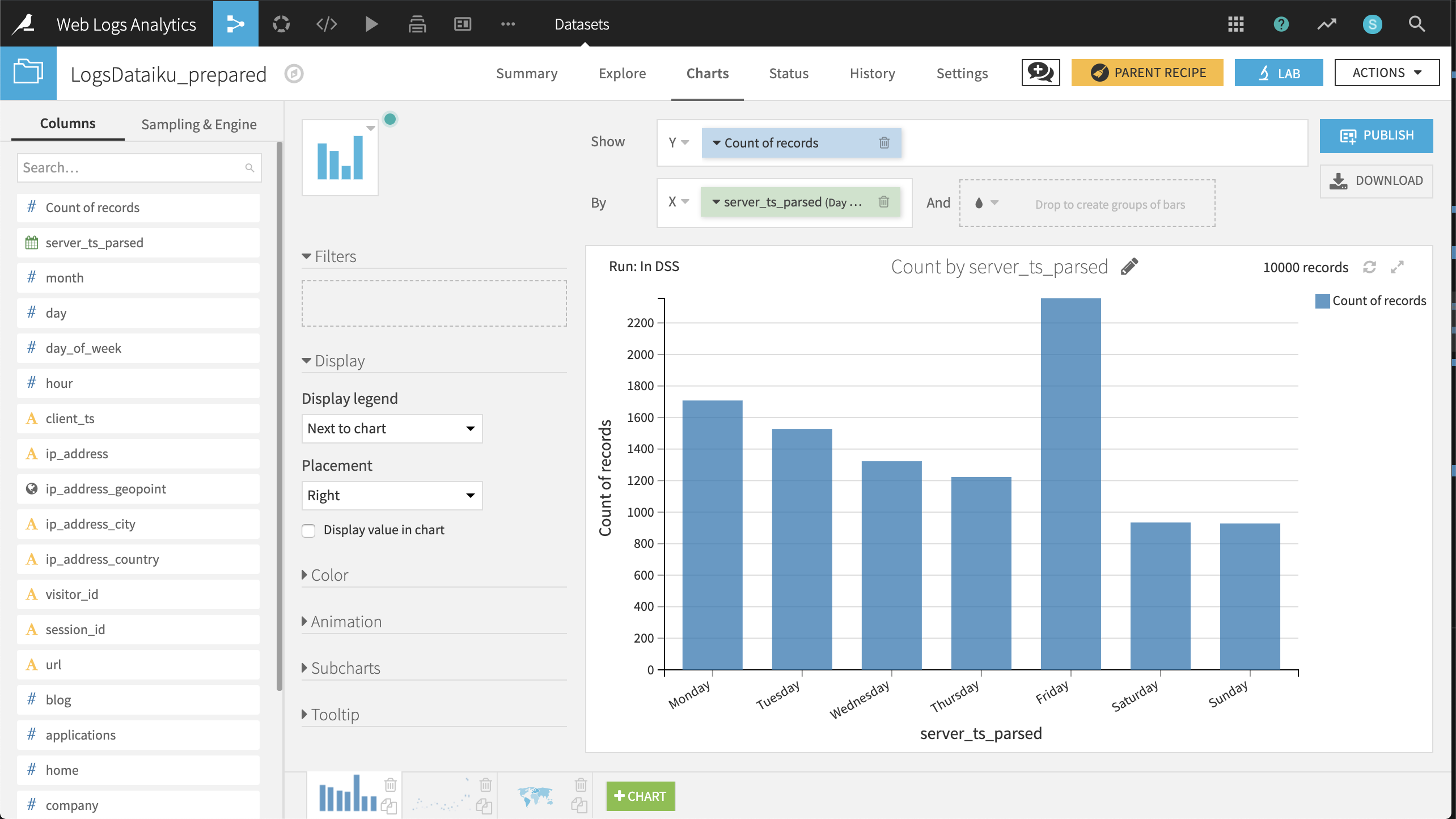
Now that our data has been cleaned and enriched, three charts can help guide our initial analysis. | - Distribution of visits by day of week.

• Create a Histogram with Count of records on the Y-axis and server_ts_parsed on the X-axis, with “Day of week” as the date range.

• The resulting chart shows that the number of visits is highest on Friday and Monday, lowest on the weekend, and visits steadily decline from Monday through Thursday before spiking on Friday.

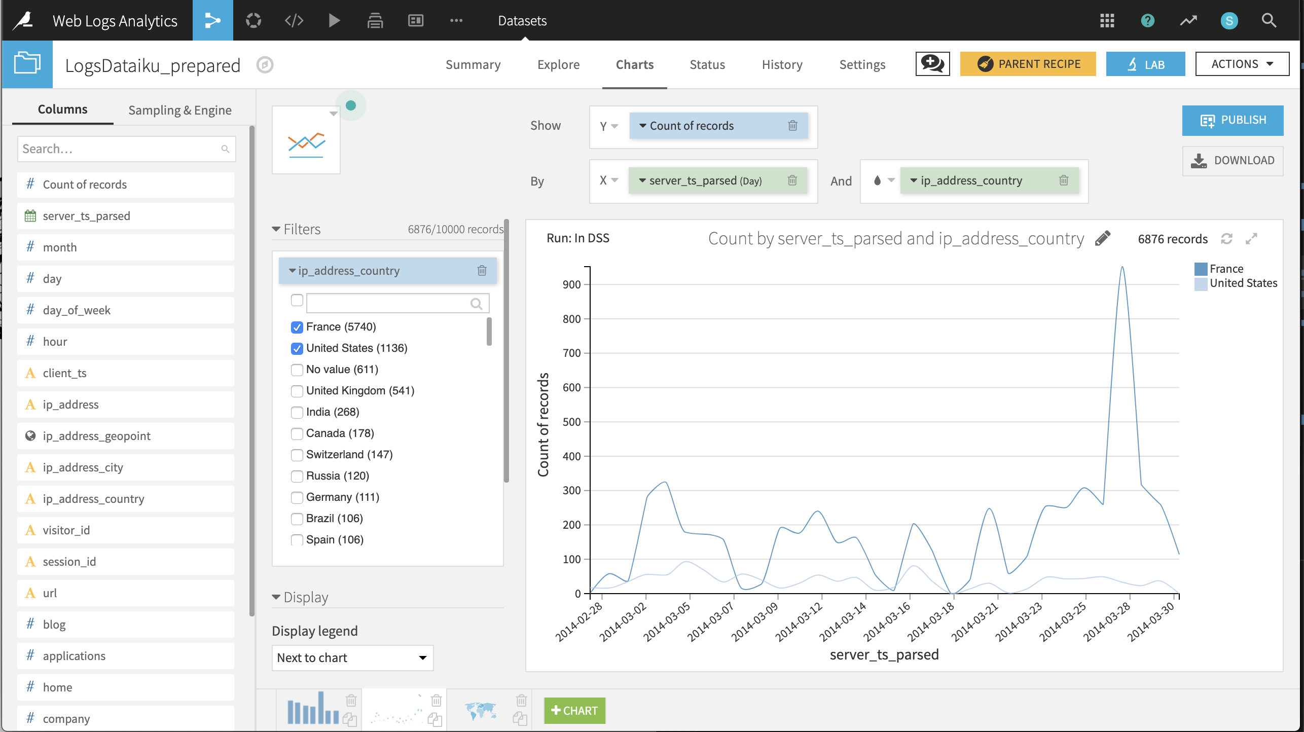
• Daily timeline of visits from France and the US

  • Create a Lines chart with Count of records on the Y-axis and server_ts_parsed on the X-axis, with “Day” as the date range.

  • Drag ip_address_country to the “And” subgroup field; plus add a filter on ip_address_country with only France and the United States selected.

  • The resulting chart suggests that, during the available period, the number of visits on any given day is highly variable; visits from France tend to outnumber those from the US; and aside from a spike on 2014-03-28, the number of daily visits is under 400.

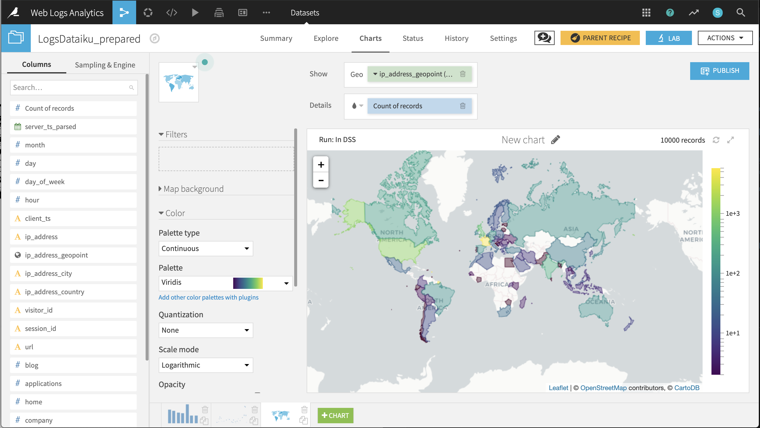
• Choropleth of visits by country of origin

  • Create a Filled Administrative Map with ip_address_geopoint providing the geographic information and Count of records providing the color details.

  • Changing the selected color palette to a multi-color palette, such as Viridis, and the color scale mode to Logarithmic can help differentiate the countries.

  • The resulting chart shows that after France and the United States, the most visitors come from the United Kingdom, India, and Canada.

Referrer Analysis

We want to identify the top referrers to the Dataiku website in terms of volume (i.e. number of pageviews and distinct visitors), as well as their level of engagement (i.e. number of distinct Dataiku URLs). In order to achieve this, we need to group the dataset by unique values within the referer_host column.

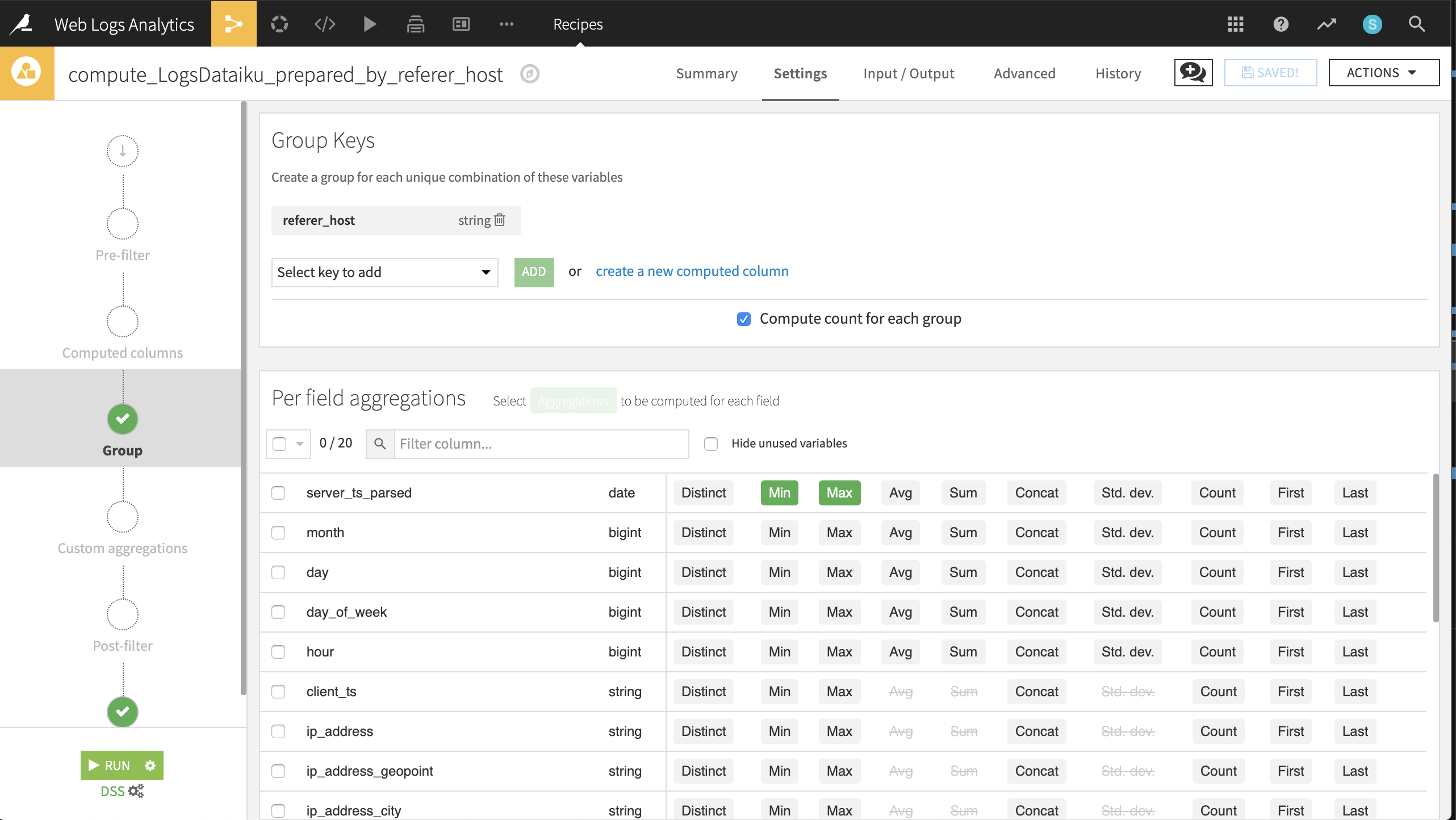
1. From the LogsDataiku_prepared dataset, create a new Group recipe with referer_host as the column to group by. Keep the default output name LogsDataiku_prepared_by_referer_host.

2. At the Group step, keep Compute count for each group selected and add the following per-field aggregations:

• For server_ts_parsed: Min, Max

• For visitor_id and url: Distinct

3. Run the recipe, updating the schema to six columns.

In the output dataset, click on the Charts tab and create the following visualizations described below. Later, we could publish these charts to a dashboard.

• Pageviews, distinct visitors and distinct URLs per referrer.

  • Create a pivot table by dragging referer_host to the rows and count, visitor_id_distinct, and url_distinct as contents.

  • referer_host should be sorted by descending order of count.

  • Keep the AVG aggregation for all of the contents.

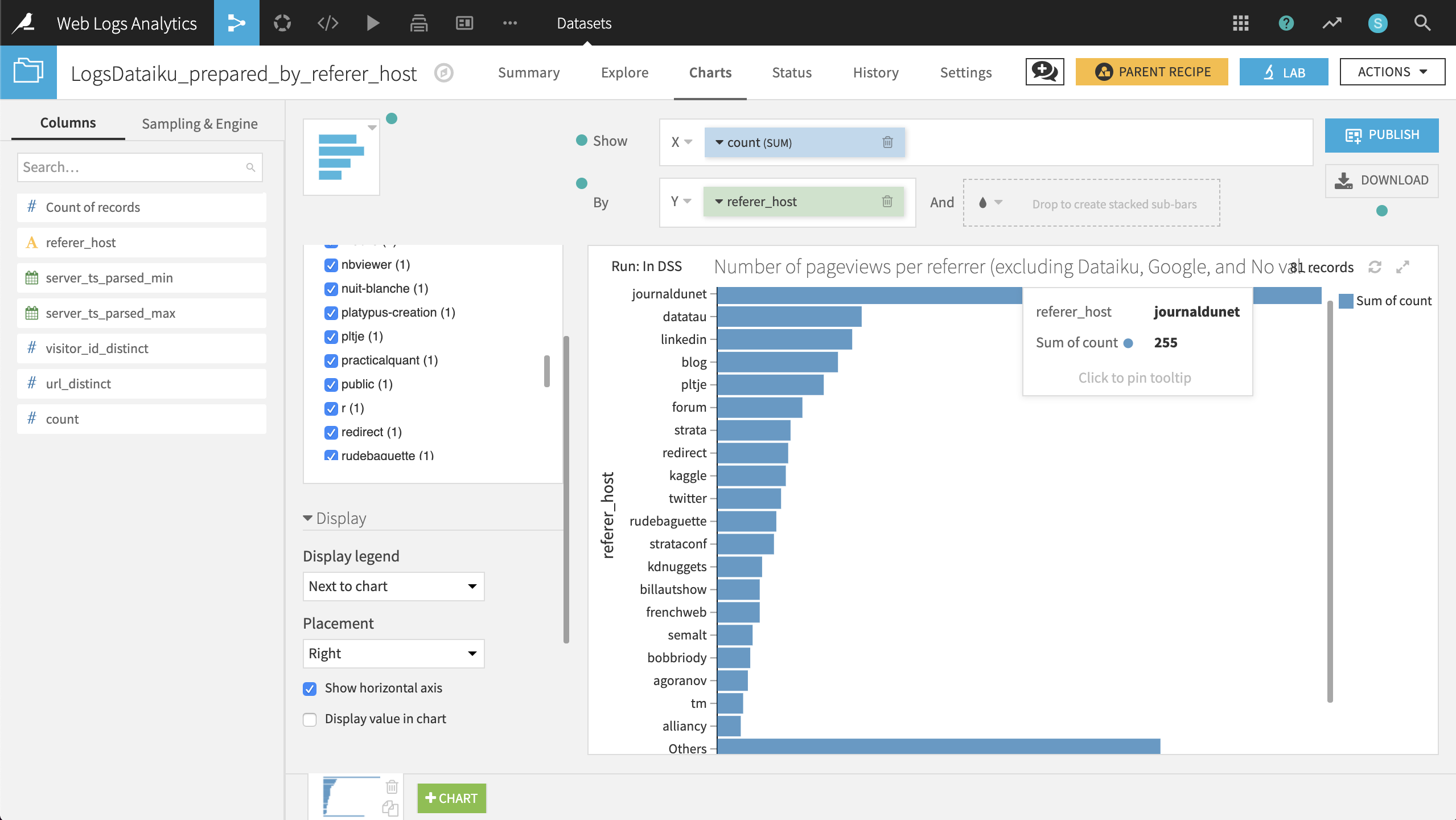
• Number of pageviews per referrer (excluding Dataiku, Google, and No value).

  • Create a bar chart with count on the X-axis and referer_host on the Y-axis.

  • count should have the SUM aggregation, and referer_host should be sorted by descending sum of count.

  • Add referer_host host as a filter, excluding dataiku, google, and No value. Under the Display menu, check the box Show horizontal axis.

  • The resulting chart shows that “journaldunet” is the largest single referrer by a wide margin.

Visitor Analysis

Now let’s attempt to segment visitors into categories and direct customers to the most appropriate channel. Our visitor analysis has the following high-level steps:

• Group visits by unique visitors

• Segment visitors using a clustering model

• Join the cluster labels with customer data

• Send the segmented data to appropriate channels for further engagement

Grouping Visitors

Using a similar technique as for referrers, we will now examine the behavior of website visitors across time (sessions).

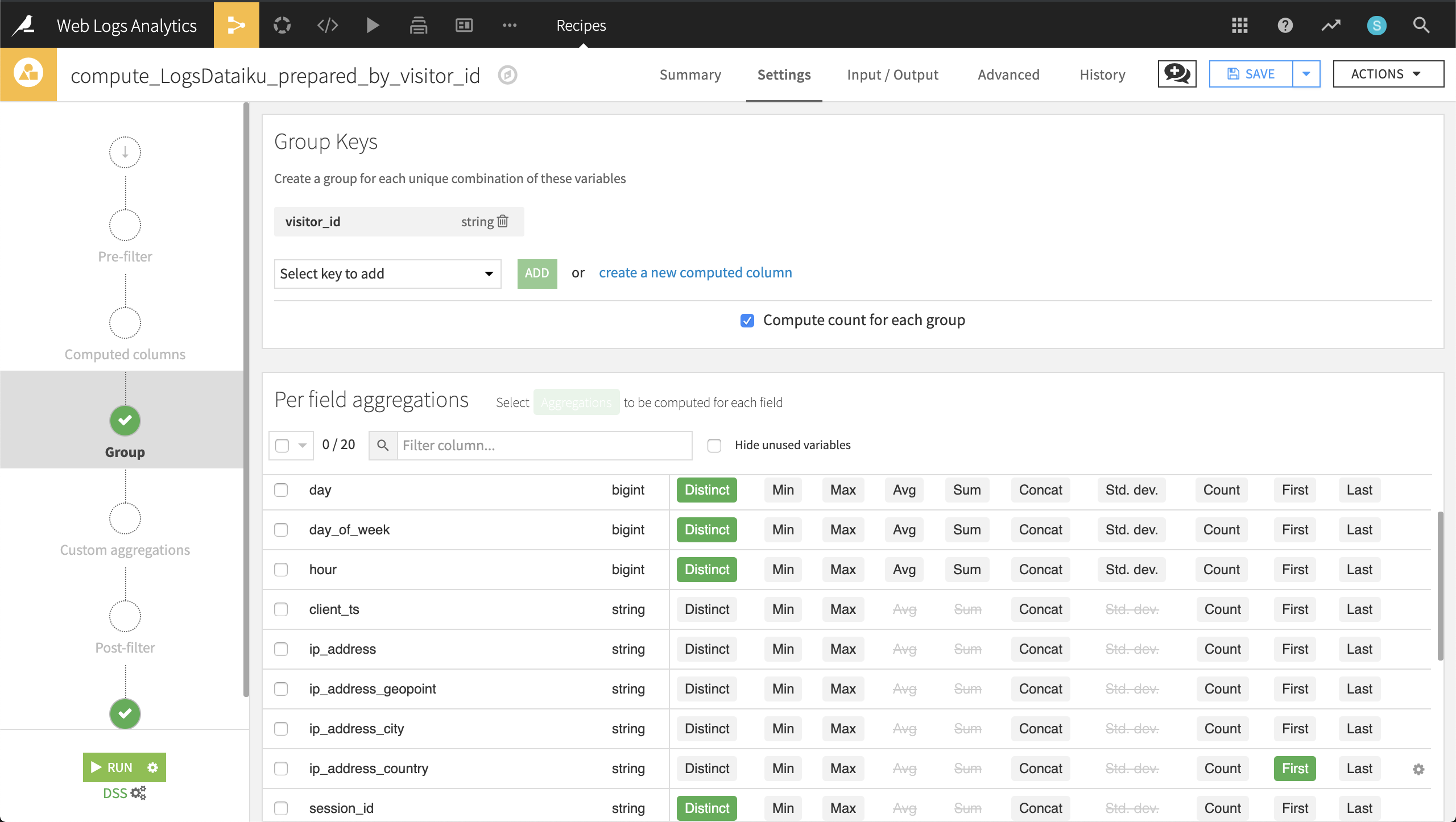
1. Returning to the LogsDataiku_prepared dataset, create a new Group recipe with visitor_id as the column to group by. Keep the default output name, LogsDataiku_prepared_by_visitor_id.

2. At the Group step, keep Compute count for each group selected, and add the following per-field aggregations:

• For day, day_of_week, hour, session_id, and url: Distinct

• For ip_address_country and user_agent_type: First

• For blog, applications, home, company, products, and data-science: Sum

3. Run the recipe, updating the schema to 15 columns.

Now for each unique visitor, we know information such as their IP address, their number of visits, the specific pages they visited, and their device (browser vs. mobile).

Clustering Web Visitors

Let’s use this data to cluster visitors into certain categories that may help our colleagues in Marketing and Sales to be more targeted in their outreach efforts.

1. From the output dataset grouped by visitor_id, go into the Lab and create a Quick Model under Visual analysis.

2. Then choose a Clustering task and, in a Quick model style, a K-Means clustering model. Keep the default analysis name.

3. Click Train to train the first model. You do not need to provide a session name or description.

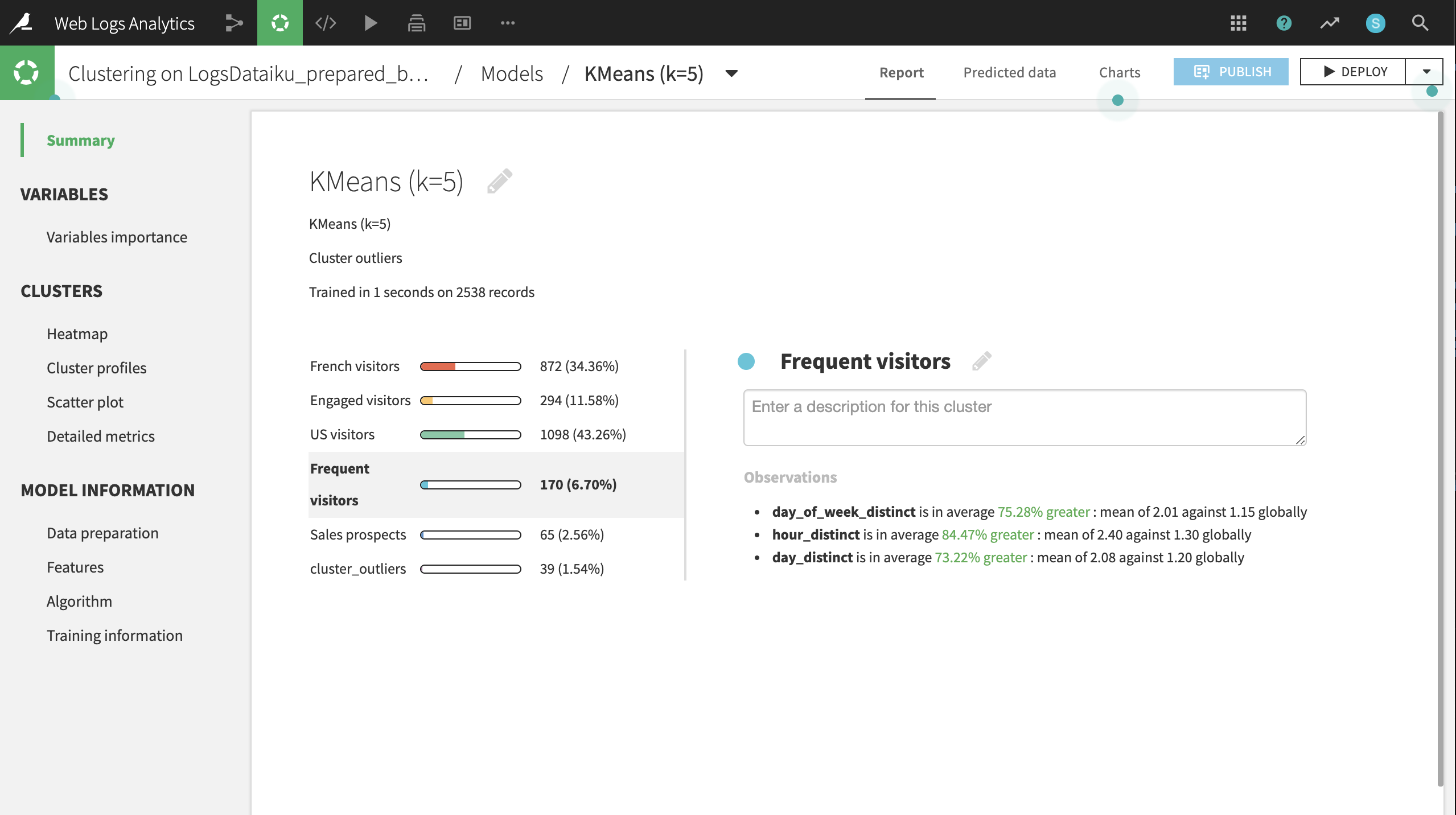
Dataiku will recognize the data types and use Machine Learning best practices when training a default clustering model. Expect the final cluster profiles to vary because of sampling effects, but there will be five primary clusters, plus a sixth cluster containing observations that do not fit any of the primary clusters.

Clicking on the model name, here KMeans (k=5), brings up the Summary tab, where you can find a wide array of model metrics and information. In the Summary tab, click the pencil icon next to each default cluster name to rename the clusters according to the suggestions below:

Cluster	Larger-than-usual numbers of:
US visitors	Americans
French visitors	French
Frequent visitors	Distinct visits
Engaged visitors	Distinct URLs visited
Sales prospects	Visits to the products page

1. From the button at the top right, Deploy the model to the Flow as a retrainable model.

2. Apply it to the LogsDataiku_prepared_by_visitor_id dataset. Keep the default model name.

3. Selecting the model from the Flow, initiate an Apply recipe. Choose LogsDataiku_prepared_by_visitor_id as the input.

4. Name the output dataset LogsDataiku_segmented.

5. Create and run the recipe.

Now, one column, cluster_labels, has been added to the output LogsDataiku_segmented.

Joining the Clusters and Customer Data

In order to map these segments to known customers, we’ll need our customer data.

1. If not already having done so, create a new UploadedFiles dataset from the customer data (CRM.csv.gz) and name it CRM.

2. From LogsDataiku_segmented, initiate a Join recipe, adding CRM as the second input. Keep the default output, LogsDataiku_segmented_joined.

3. In the Join step, visitor_id should be automatically recognized as the join key. Change the type of join to an Inner Join to keep only records where a customer can be successfully matched with website visits.

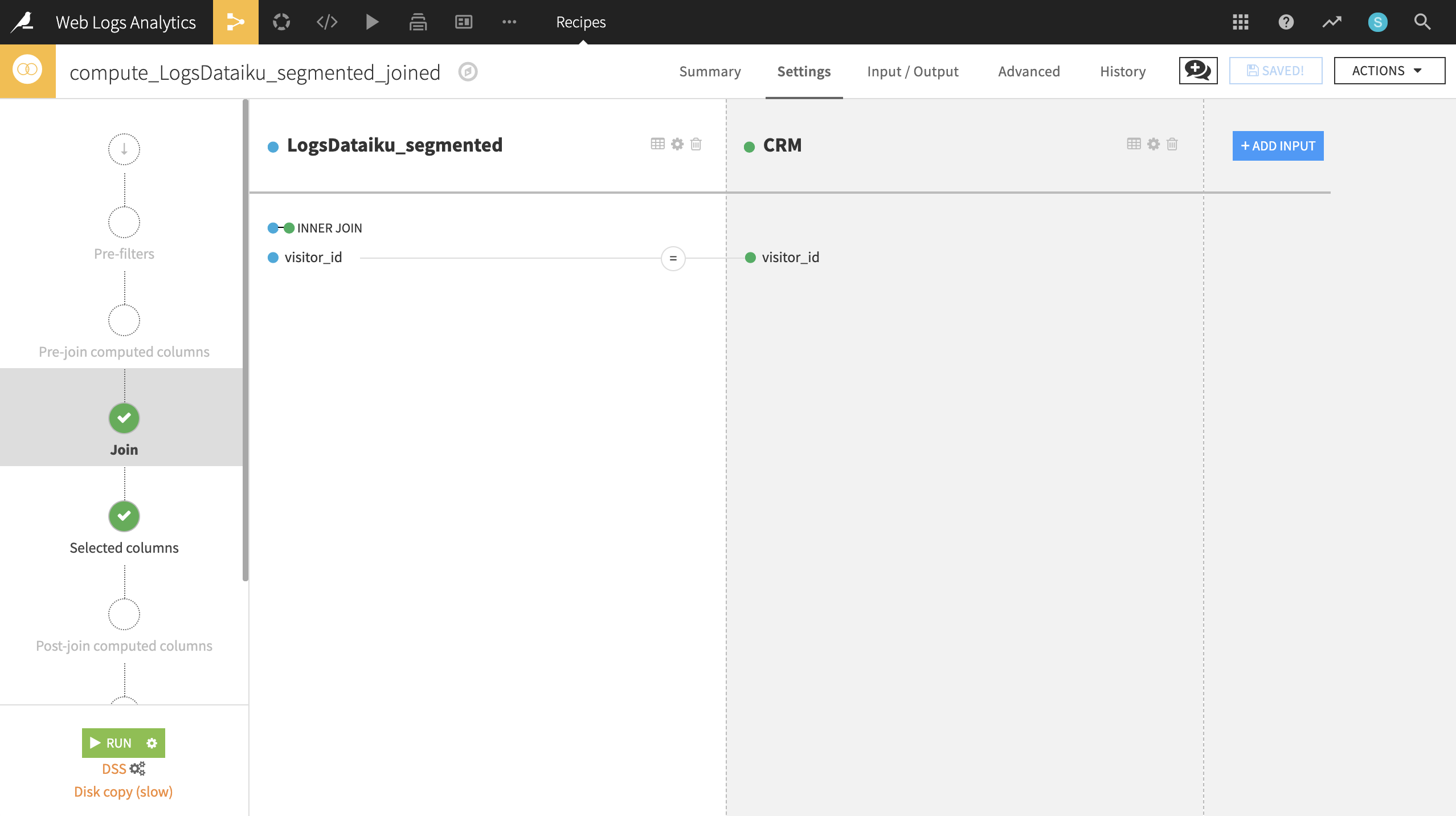
After completing the join, expect an output of 5602 rows and 35 columns.

Customizing and Activating Segments

Now we want to feed these customers into the right channel: Marketing, Prospective Sales, or Sales.

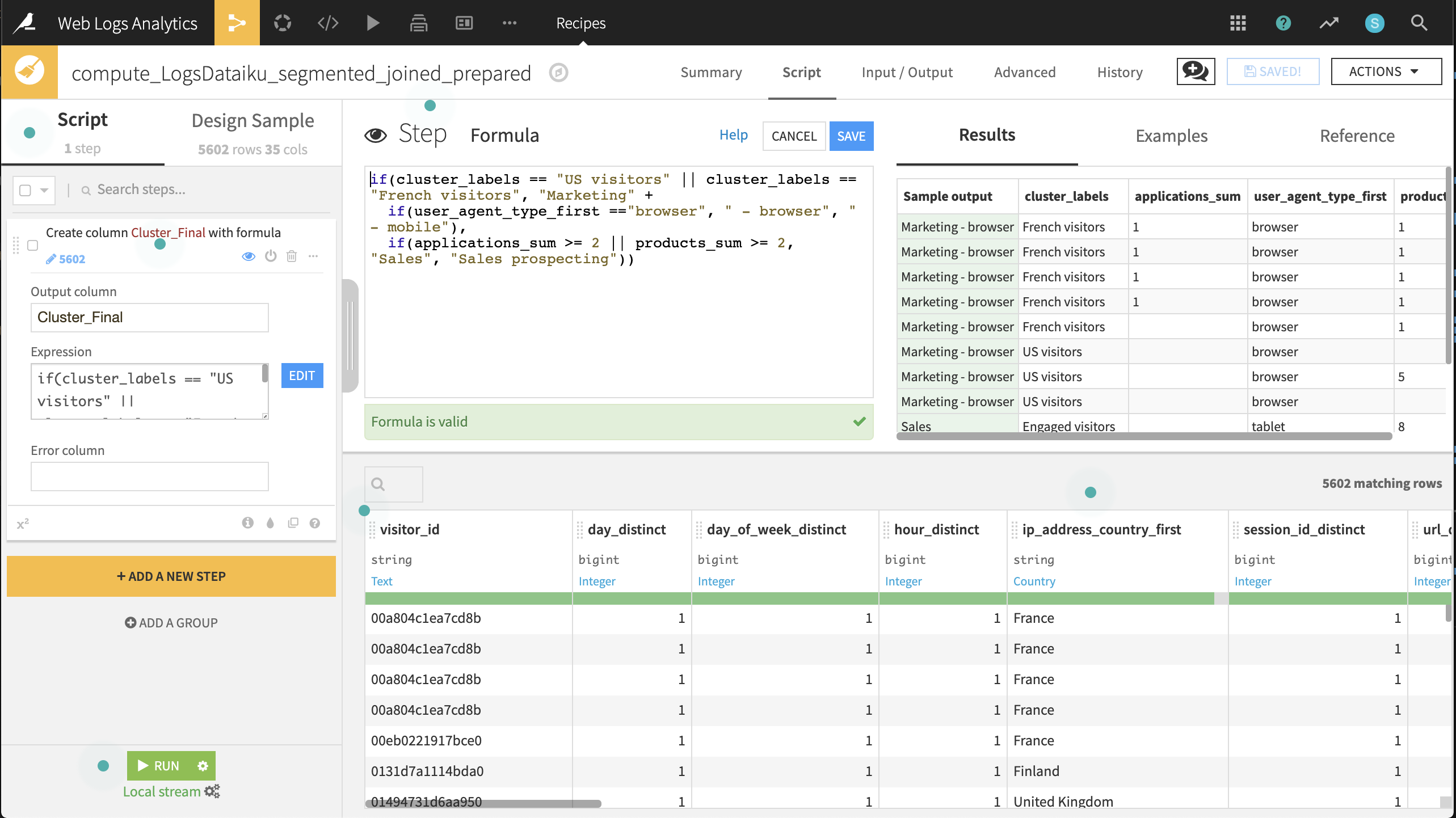
1. Create a Prepare recipe from the LogsDataiku_segmented_joined dataset. Keep the default output name.

2. Add a new step with the Formula processor creating a new column, Cluster_Final, using the expression defined below:

if(cluster_labels == "US visitors" || cluster_labels == "French visitors", "Marketing" +
  if(user_agent_type_first =="browser", " - browser", " - mobile"),
  if(applications_sum >= 2 || products_sum >= 2, "Sales", "Sales prospecting"))

3. Run the recipe, updating the schema to 36 columns.

Now let’s split the dataset on this newly created variable so we can ship the smaller subsets to the right teams.

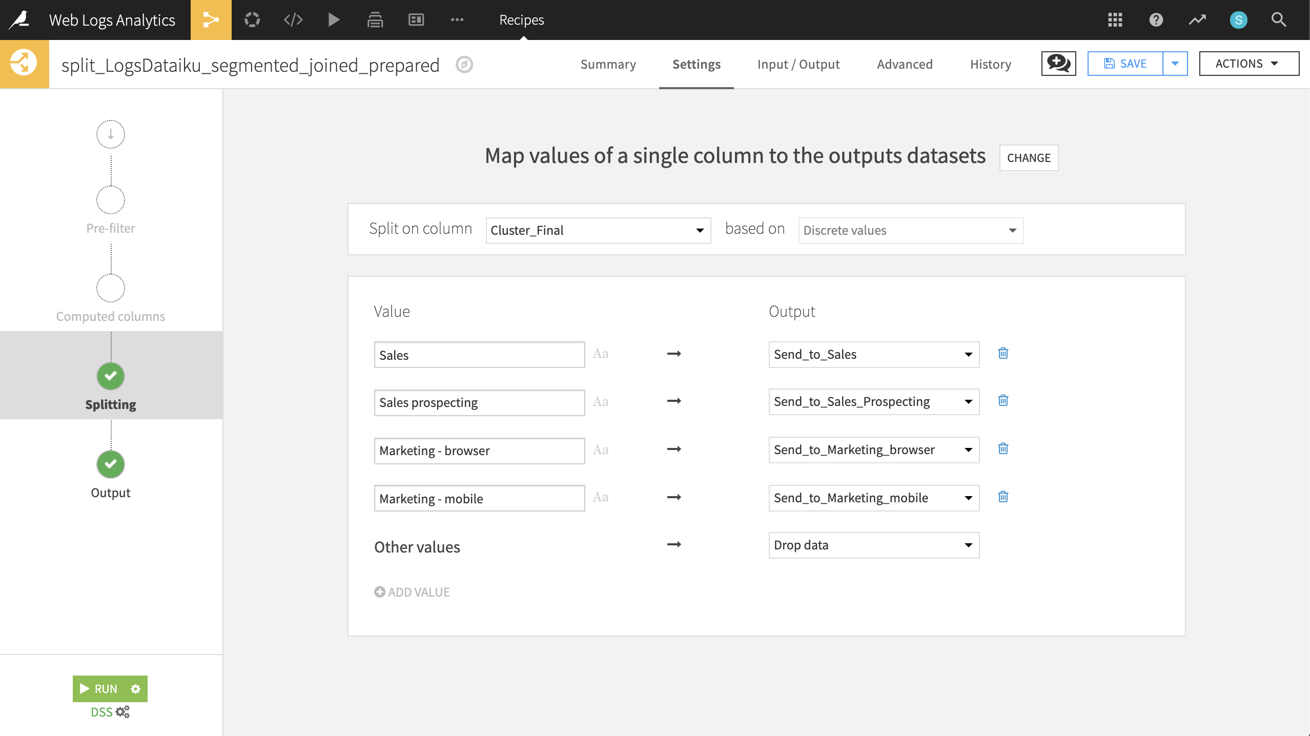
1. From the output dataset, LogsDataiku_segmented_joined_prepared, create a Split recipe that sends each of the four values of Cluster_Final to individual datasets. Use the names:

• Send_to_Sales

• Send_to_Sales_Prospecting

• Send_to_Marketing_browser

• Send_to_Marketing_mobile

2. Choose Map values of a single column as the Splitting method.

3. Choose Cluster_Final as the column on which to split.

4. Add the values and outputs according to the screenshot below.

5. Run the recipe.

These newly generated datasets are immediately usable by customer-facing team members to send targeted emails!

Wrap-up

Congratulations! We created an end-to-end workflow to build datasets as collateral for colleagues in Sales and Marketing. Thank you for your time working through this use case.

Remember, you can always refer to the completed project in the Dataiku gallery.