Interpreting Regression Models’ Outputs

If you want to turn your predictive models in a goldmine you need to know how to interpret the model quality assessment provided by DSS. It can get complicated because the error measure to take into account may depend on the business problem you want to solve. Indeed to interpret and draw most profit from your analysis you have to understand the basic concepts behind error assessment. And even more importantly, you have to think about the actions you will take based on your analysis.

In this post we will go through metrics given when you use a regression model in DSS and how to interpret them in terms of business application.

As an illustration we will use the Boston housing dataset. It’s a classic as machine learning textbook datasets go and it’s also a business application. The target we want to predict is house pricing as a function of features such as the number of teacher per children or the distance to employment hubs. Finding the right price is essential to find a buyer in reasonable time and at the best price.

Upload the Boston Housing dataset in DSS, open an analysis on the dataset and create a first prediction model with the price as target feature. DSS will automatically train two models on the dataset and display them in a list.

Actual vs predicted values scatterplot

When you ask DSS to train a model, it begins by splitting your dataset into train and test sets. Click on a model in the list and select the training information tab:

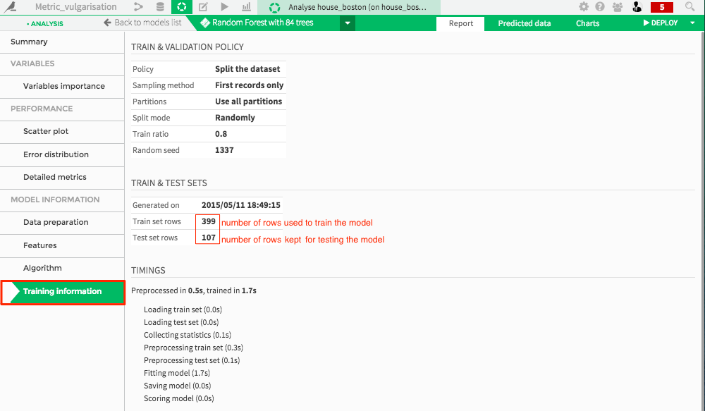
DSS optimizes model parameters on the train set and keeps the test set for assessing the model.

Head to the scatter plot tab, for each point in the test set, the graph displays the actual value of the target on the x-axis, and the value of the target predicted by the model on the y-axis.

If the model was perfect, all points would be on the diagonal line. This would mean that predicted value are exactly equal to actual values. The error on a datapoint is the vertical distance between the point and the diagonal. The point below the diagonal line are underestimated by the model and points above it are overestimated.

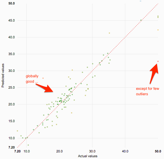
You want to minimize the distance from the points to the diagonal (hence the error). However for some applications, overestimating can be way more problematic than underestimating.

An example would be predictive maintenance: Imagine you own a truck company and want to know when trucks are going to encounter failures. You want to repair them ahead of time, when there are at the garage and prevent failures from happening while on duty.

In this case, you should underestimate the time left before a failure happens to be sure to act on it properly. Overestimating means you won’t repair trucks in time and that model would be useless. This perfectly illustrates the effect that errors can have when they are not symmetric.

Global scores

On the model list page, there is a field with an indicator that is a global measure of how good your model is. DSS provides you with all the standard statistical scores.

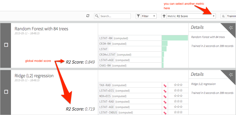
Explained Variance Score, R2 score and Pearson correlation coefficient should be compared to 1 (the closer to 1 the better the model is). The other ones (Mean Absolute Error, Mean Absolute Percentage Error, Mean Squared Error, Root Mean Squared Error, Root Mean Squared Logarithmic Error) are error measures and should be as close as possible to zero.

If you click on a model and open the detailed metrics tab you will have a list of scores. Each score is shortly defined. You can refer to wikipedia entries for the detailed definitions of these scores.

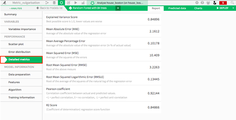
Here we will go through the scores, give an interpretation, and develop, if possible, an implication in terms of business.

• Pearson coefficient: Correlation is computed between two variables and assesses to what extent the variables vary simultaneously. If the variables increase at the same time they are said to correlate. Inversely, if one variable increases while the other decreases, they anti-correlate. In our case, the correlation coefficient is computed between the predicted and the actual values. Hence, the closer the correlation is to 1, the better the model.

• R2 (coefficient of determination) is the square of the Pearson coefficient.

• Explained Variance Score: It gives you the fraction of what your model is able to explain of your target. If you may, it’s the fraction of what the model knows compared to all there is to know about your target.

• Mean Squared Error and Root Mean Squared Error: The variance of the error and the standard deviation of the error. If the model error is normally distributed (check the error distribution to know that), multiplying the standard deviation by three, you will obtain a very safe interval of how big your error can be. The problem with this error is that it is very sensitive to outliers. This means that if you have a very good model with a large error only for one datapoint (that might be a measurement error) this score will be high.

• Mean Absolute Error (MAE): An alternative to the outlier sensitive MSE is the MAE. Because it takes the absolute value of the error, the effect of one outlier won’t be as drastic than for RMSE.

• Mean Average Percentage Error is an interesting metric. Instead of measuring the simple discrepancy between predicted values and actual values it gives the error in percentage of the value itself. This means that an error of 10,000$ on a flat costing 200,000$ is considered equivalent to an error of 100,000$ on a mansion costing 2,000,000$. This seems particularly appropriate for pricing targets.

• Construct your custom metric: the metric above makes sense in most cases but depending of what you want to do you may need to create a custom metric. Going back to our predictive maintenance example with trucks, you could implement a score that is the global price of repairs for the next year. Every time your model predicts the failure before it happens, your cost is a simple repair. However if the predicted failure happens after the actual failure you will pay for the repair and the price of retrieving the truck! Of course you don’t want to put your truck in repairs every two days. So your score should take the frequency of interventions on a single truck into account.