Hands-On: Standard Webapp
In this tutorial, you will learn how to create a webapp in Dataiku DSS, using HTML, JavaScript, CSS, and a Python backend, to display two interactive charts which will update based on user input.
Let’s Get Started!
To create the webapp, we will use data from the fictional Haiku T-shirt company, which was also used in the Basics tutorials.
Prerequisites
Some familiarity with HTML and JavaScript;
Some familiarity with Python (to use the Python backend);
Internet access (to call the most recent web-hosted versions of certain libraries in the code).
Technical Requirements
An instance of Dataiku DSS - version 8.0 or above (Dataiku Online can also be used);
A Python code environment with the mandatory packages installed.
Note
If you are using Dataiku Online, you can use the “dash” code environment. Otherwise, you can follow the instructions in this article to create a code environment compatible with all courses in the Developer learning path.
This tutorial was tested using a Python 3.6 code environment. Other Python versions may be compatible.
Tip
If you are NOT following this tutorial as part of the Developer learning path, you can use the DSS builtin code environment, which has all the mandatory packages.
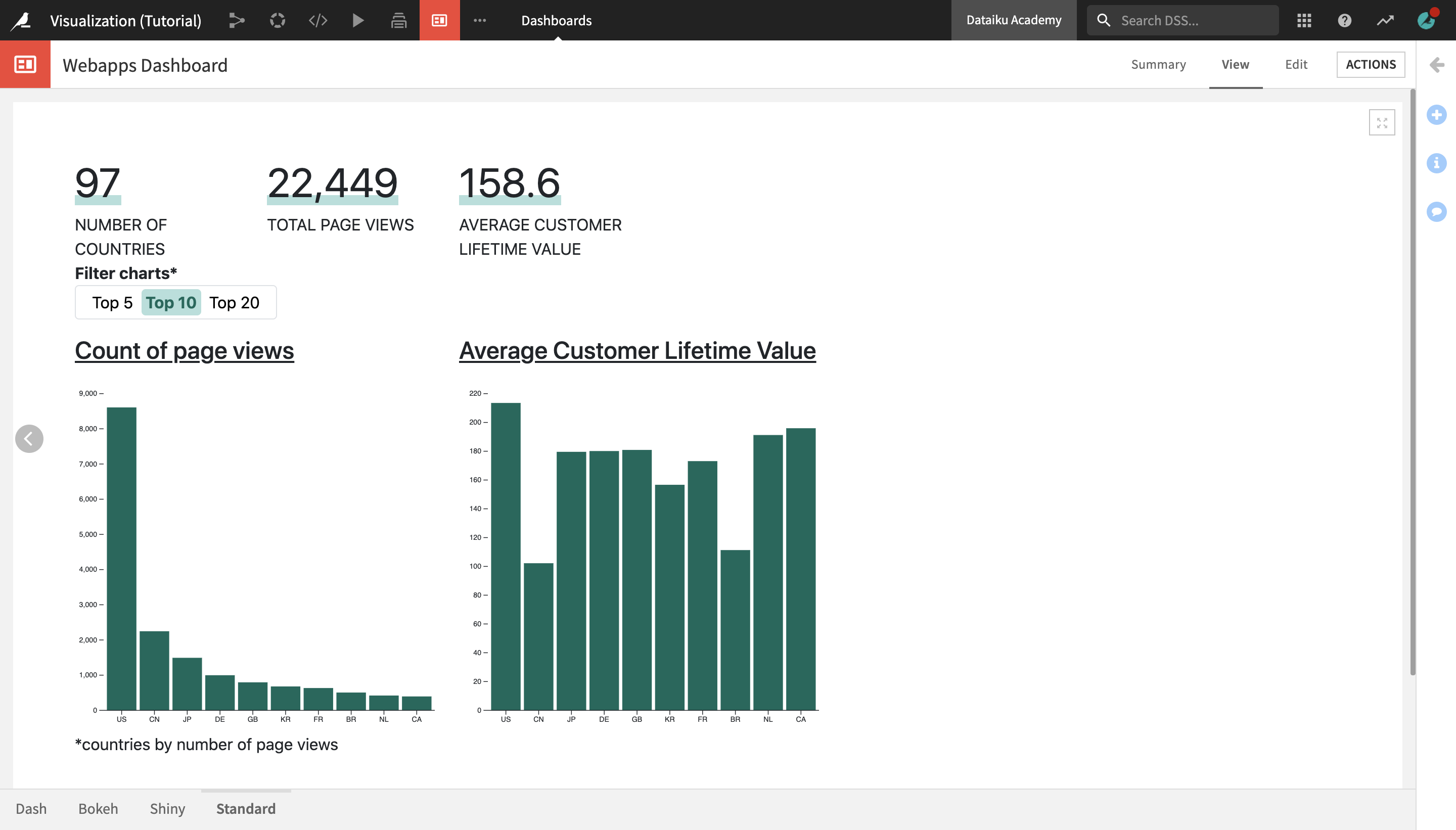
Webapp Overview
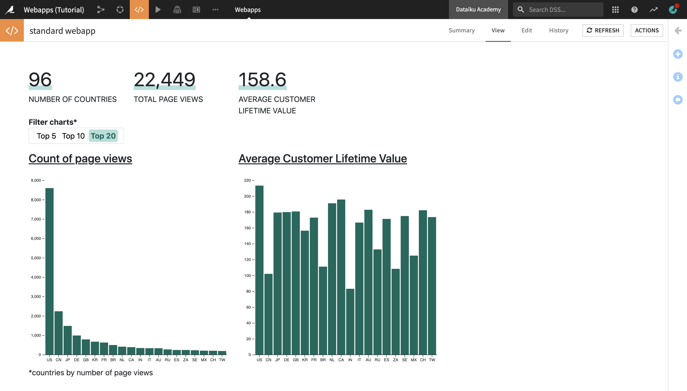
The webapp will visualize the countries with the highest number of page views, and their average customer lifetime value. It will let the users choose to display the top 5, 10, or 20 countries.
The results of the finished webapp are shown below.
Create Your Project
Create your project by selecting one of these options:
Import a Starter Project
From the Dataiku homepage, click +New Project > DSS Tutorials > Developer > Visualization (Tutorial).
Continue From the Previous Hands-On Tutorial
If you are following the Academy Visualization course and have already completed one of the previous hands-on lessons, you can begin this lesson by continuing with the same project you created earlier.
Download and Import Dataset Into New Project
Alternatively, you can download the revenue_prediction dataset and import it into a new project.
Create a New Standard Webapp
To create a new Standard webapp:
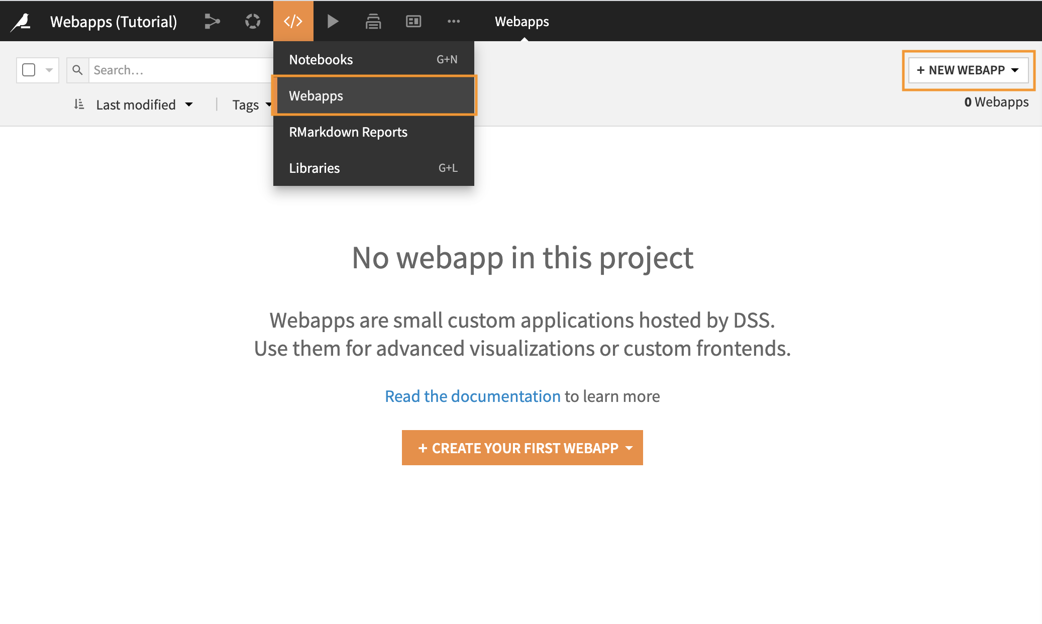
In the top navigation bar, select Webapps from the Code (</>) menu.
Click + New Webapp > Code Webapp > Standard.
From the displayed options, select Simple webapp to get started.
Type a simple name for your webapp, such as
standard webapp, and click Create.
You will land on the Edit tab of the webapp.
Explore the Webapp Editor
The webapp editor is divided into two panes.
The left pane allows you to see and edit the Python code underlying the webapp. It contains tabs for each language: HTML, CSS, JavaScript (JS), and Python.
The right pane gives you several views on the webapp:
The Preview tab allows you to write and test your code in the left pane while having immediate visual feedback in the right pane. At any time you can save or reload your current code by clicking on the Save button or the Reload Preview button.
The HTML, CSS, JavaScript (JS), and Python tabs allow you to look at different portions of the code side-by-side in the left and right panes.
The Log is useful for troubleshooting problems.
The Settings tab allows you to set the code environment for this webapp, if you want it to be different from the project default.
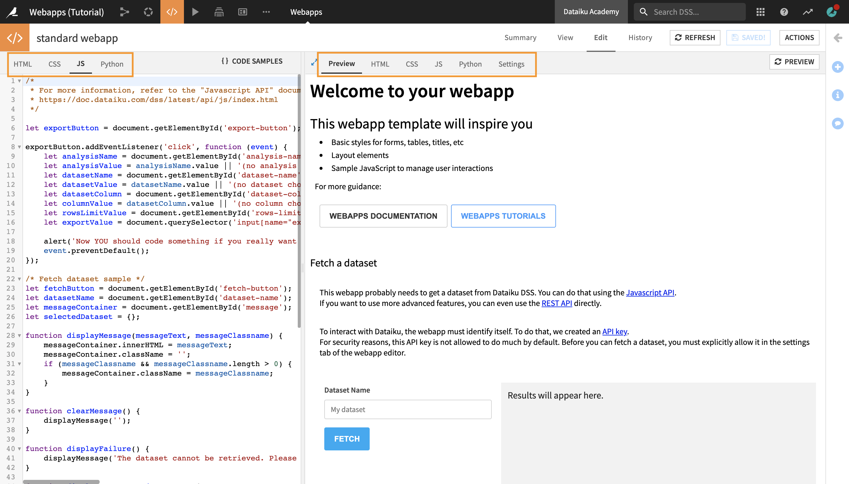
A webapp template with some pre-written sample code will appear. This can be useful to start from when creating a new webapp, but for the purpose of this tutorial, we will start from scratch.
Delete the sample code in the HTML, CSS, and JS tabs.
Click Save in the upper right corner of the page.
The Preview tab now displays an empty page.
Change the Settings
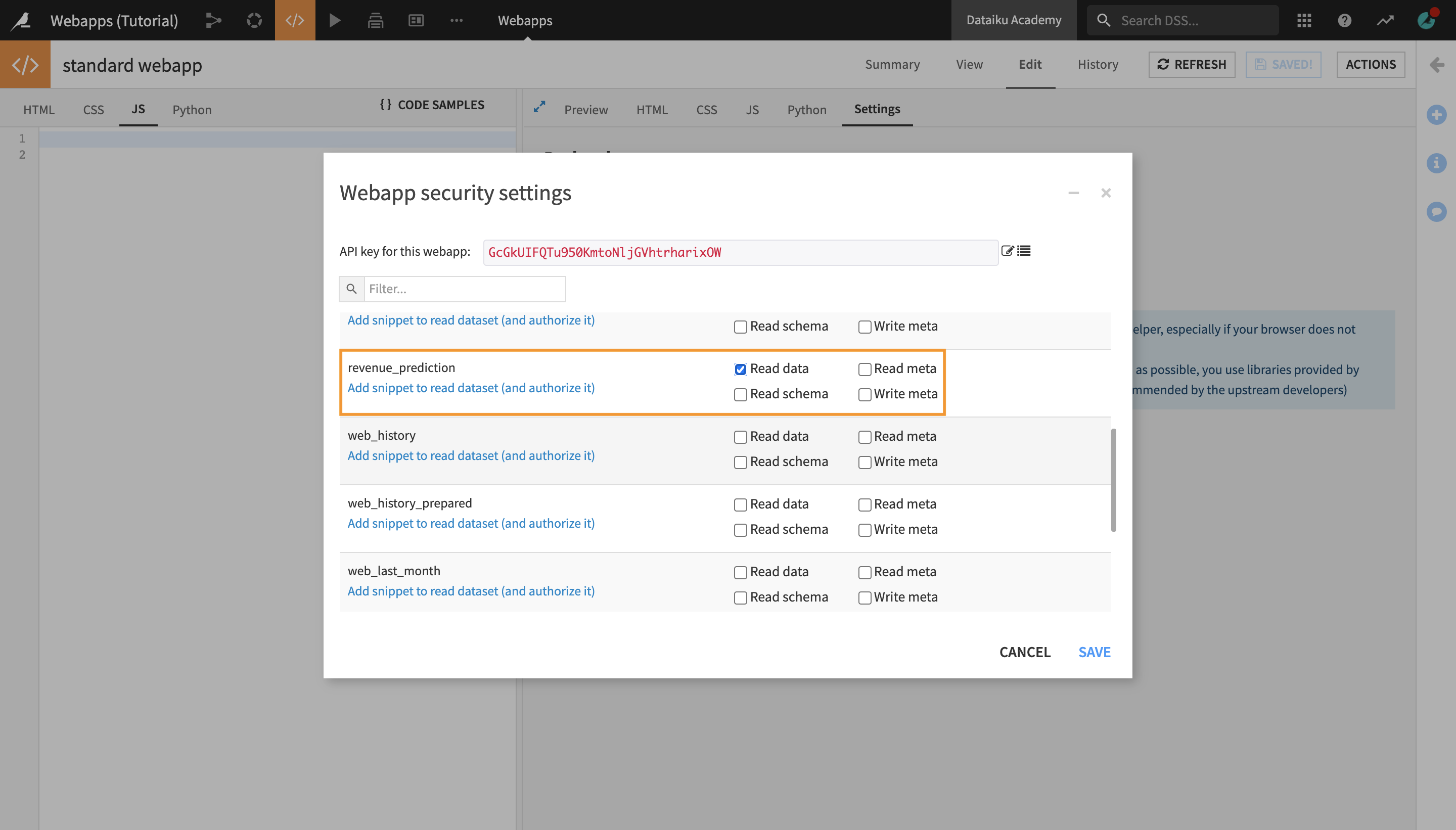
Since we will be reading a dataset from the Flow, we first need to authorize it in the security settings.
Navigate to the Settings tab in the webapp editor.
Click Configure under the Security heading.
Select Read data for the revenue_prediction dataset.
Click Save.
In the Settings tab, you will also find JavaScript libraries that you can import.
Note
The JavaScript libraries you see in this section are installed within Dataiku DSS, meaning that you don’t require internet access to load them. However, some of them might be older versions. In this hands-on, we will use the most up-to-date versions that we will call directly in HTML, using web-hosted versions.
In addition, we are going to use the JavaScript library D3.js (version 6) to visualize the charts, and the Bootstrap framework (version 5). We will call them from the HTML code at a later point in this tutorial (you do NOT need to add these in the Settings tab).
Return to the Preview tab.
Code the Webapp
Let’s build the code behind the Standard webapp.
Set Up the Backend
First, we will send a prepared dataset to the frontend.
Navigate to the Python tab in the left side pane.
Click Enable to enable the Python backend for this webapp.
Note
The Python backend is in Flask, a powerful micro web framework. It makes it possible to set up routes to communicate with the frontend. On top of this, the Python backend makes it possible to fetch our dataset from the Flow and manipulate it.
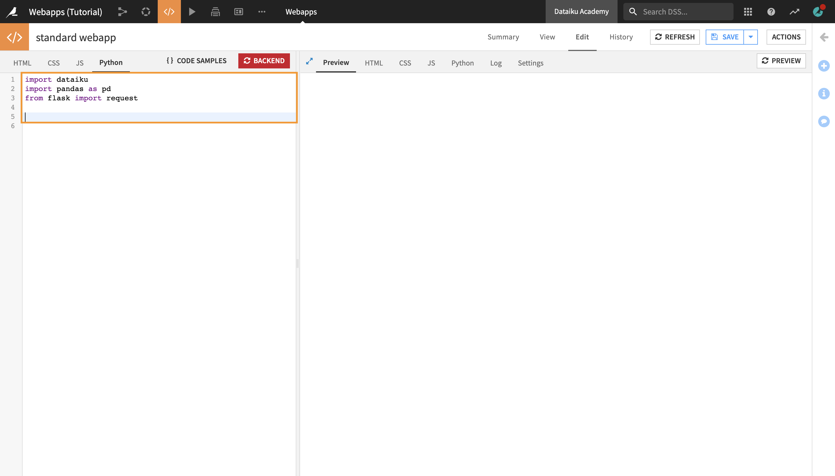
Once the Python backend is enabled, the webapp editor displays a piece of sample starter code. This is useful when starting to write a new webapp, but as we are starting from scratch, we can delete everything except for the import functions at the top:
Delete the sample code, except for the first three lines.
Now, let’s write the code to set up the backend and the data.
The Python code below will:
import required libraries;
get the dataset from the Flow and convert it into a Pandas dataframe;
aggregate the data in a way that will make it easy to display the top countries;
set up a route which will be callable by the JavaScript frontend with
/send_data;define a function which will return the data as JSON.
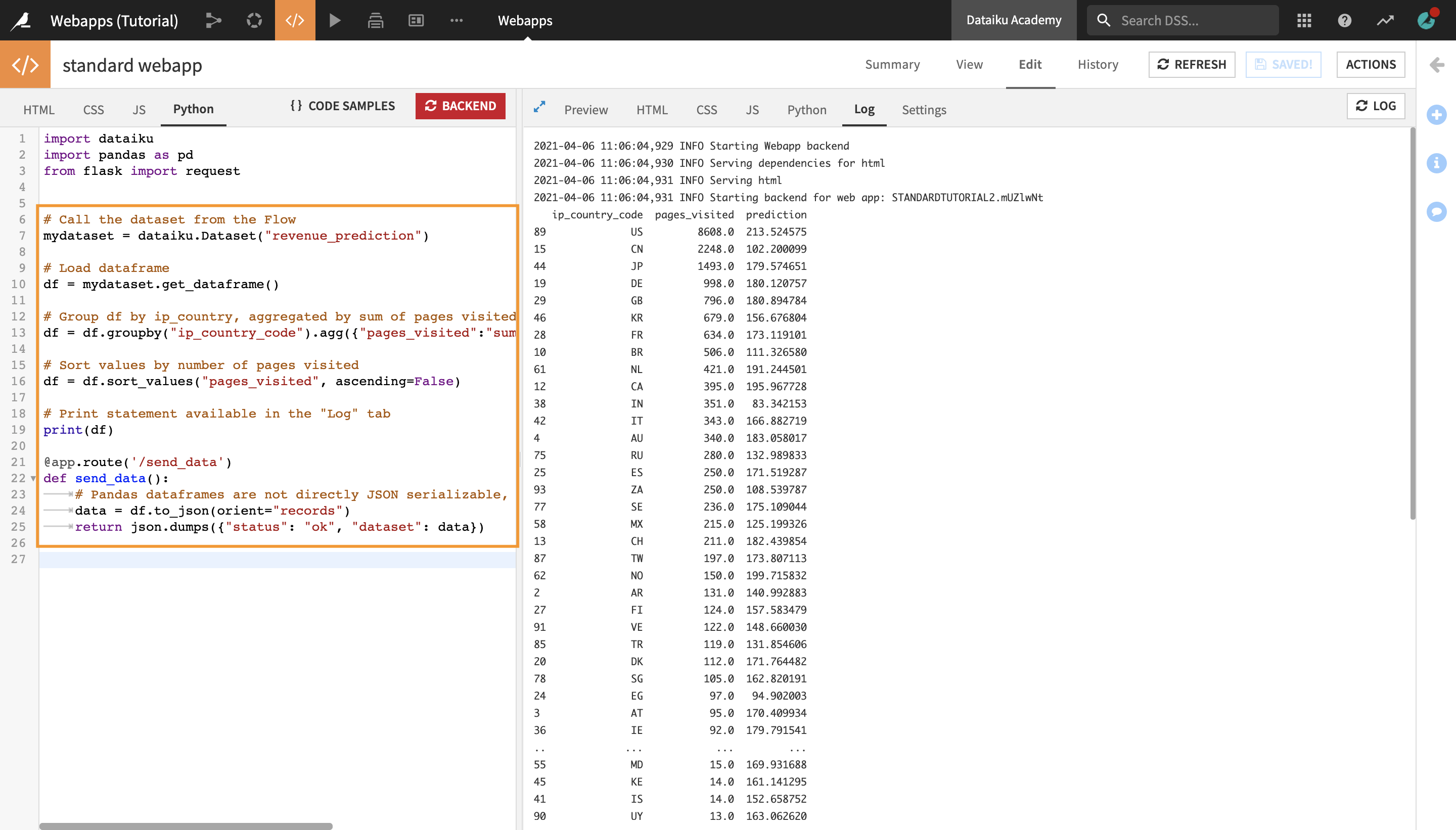
Enter the code below in the Python tab of the webapp editor, after the three first lines (the import functions that we retained from the sample code).
# Call the dataset from the Flow
mydataset = dataiku.Dataset("revenue_prediction")

# Load dataframe
df = mydataset.get_dataframe()

# Group df by ip_country, aggregated by sum of pages visited and average of prediction
df = df.groupby("ip_country_code").agg({"pages_visited":"sum","prediction":"mean"}).reset_index()

# Sort values by number of pages visited
df = df.sort_values("pages_visited", ascending=False)

# Print statement available in the "Log" tab
print(df)

@app.route('/send_data')
def send_data():
    # Pandas dataframes are not directly JSON serializable, use to_json()
    data = df.to_json(orient="records")
    return json.dumps({"status": "ok", "dataset": data})
Click Save.
To check the Python code, we also added a print statement. Its results appear in the Log tab.
Navigate to the Log tab in the right side to see the printed dataframe.
Retrieve the Data in the Frontend With JavaScript
Next, let’s retrieve the data in the frontend with the send_data() function.
In the JS tab, we will replace the existing starter code with the function below to:
call the
send_data()function from the backend;check in the data if the code is returned.
To get the data, we will use the jQuery method $.getJSON() with the dataiku function getWebAppBackendUrl() to retrieve the URL of our webapp, with the route we are interested in.
From there, we will pass the data variable which will fetch the data return in our “send_data()” backend function, and then log it.
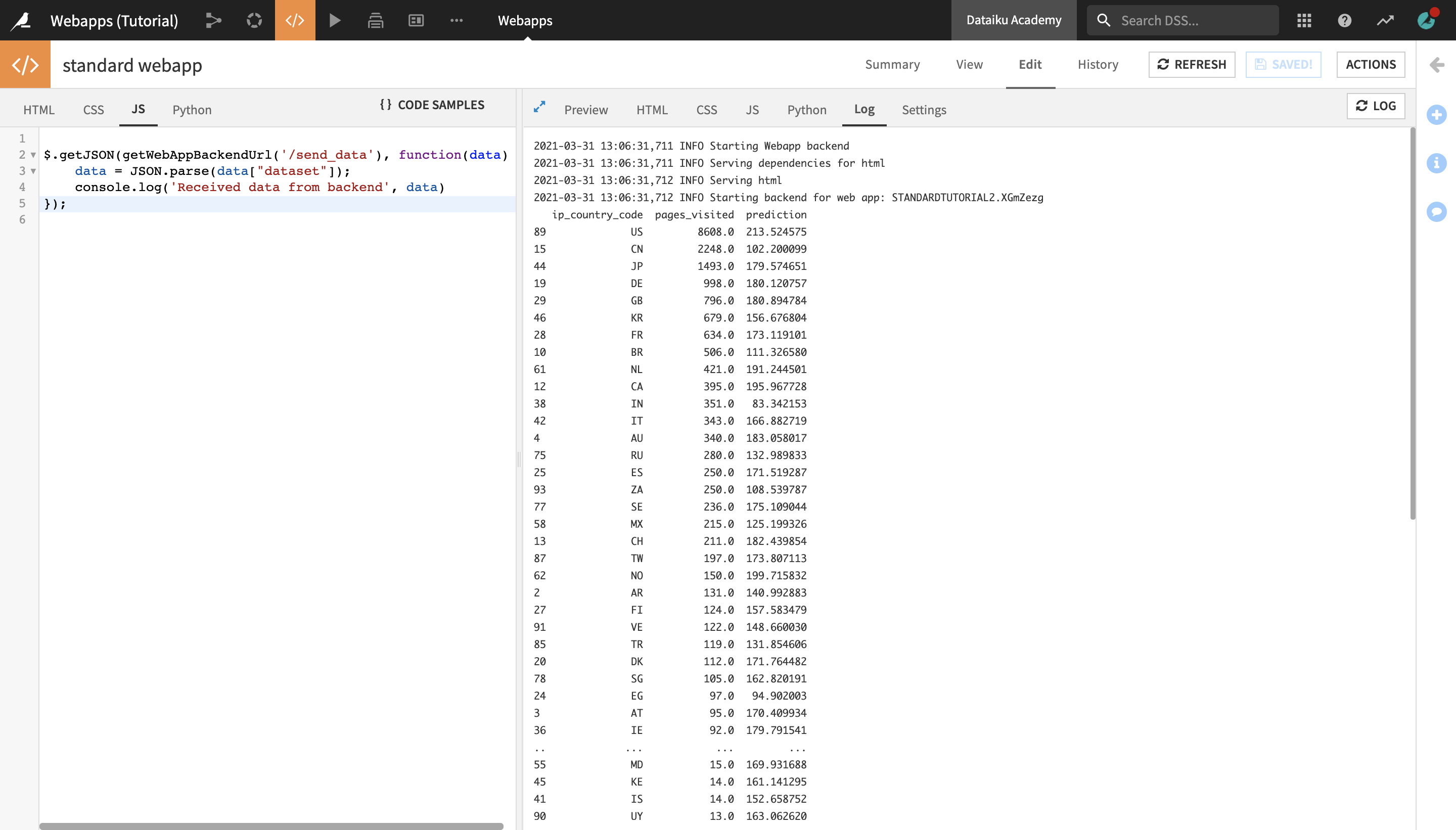
Replace the existing starter code with the one below:
$.getJSON(getWebAppBackendUrl('send_data'),function(data){
    data = JSON.parse(data["dataset"]);
    console.log("our data", data);
})
Open the Log.
You should get an array of 96 objects with the ip_country_code, pages_visited and prediction keys.
Design the UI With HTML and Bootstrap
In this section, we will use HTML and the Bootstrap framework in order to design the UI of our webapp. Bootstrap allows us to assign CSS classes which have already been developed.
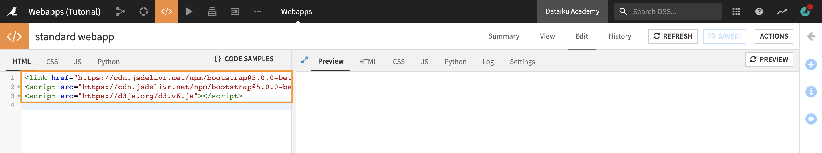
We’ll start by importing Bootstrap and d3.js directly in the HTML code.
Navigate to the HTML tab of the webapp editor and enter the following code:
<link href="https://cdn.jsdelivr.net/npm/[email protected]/dist/css/bootstrap.min.css" rel="stylesheet" integrity="sha384-giJF6kkoqNQ00vy+HMDP7azOuL0xtbfIcaT9wjKHr8RbDVddVHyTfAAsrekwKmP1" crossorigin="anonymous">
<script src="https://cdn.jsdelivr.net/npm/[email protected]/dist/js/bootstrap.min.js" integrity="sha384-ygbV9kiqUc6oa4msXn9868pTtWMgiQaeYH7/t7LECLbyPA2x65Kgf80OJFdroafW" crossorigin="anonymous"></script>
<script src="https://d3js.org/d3.v6.js"></script>
Click Save.
Next, we will design the layout.
There are several things to keep in mind:
We will insert Bootstrap classes in our HTML code, without having to code the CSS;
We will add specific IDs to our code in order to call them later in the JavaScript code with d3.js;
Later, we will add a few classes and specify some additional styling with CSS on top of Bootstrap;
All the data points, including metrics and charts, will be built in the JavaScript code.
There will be:
one Bootstrap container to wrap the dashboard altogether;
three rows: one with metrics, one with inputs clickable by the user, and one for our two charts;
- columns to properly divide the page:
Bootstrap divides the page in 12 columns;
Col-X will take the space of X columns.
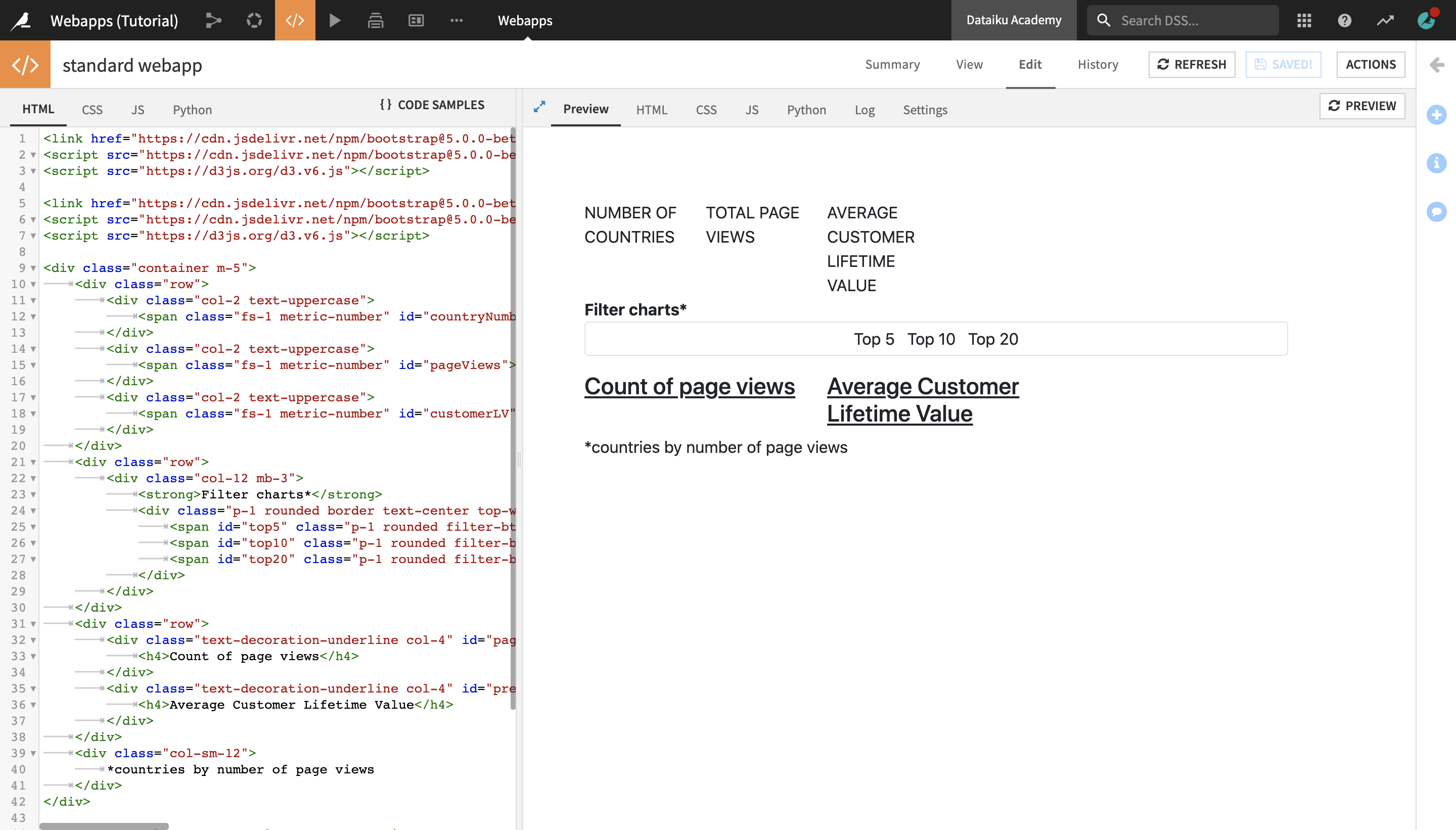
Enter the following code in the HTML tab of the webapp editor, beneath the existing three lines:
<link href="https://cdn.jsdelivr.net/npm/[email protected]/dist/css/bootstrap.min.css" rel="stylesheet" integrity="sha384-giJF6kkoqNQ00vy+HMDP7azOuL0xtbfIcaT9wjKHr8RbDVddVHyTfAAsrekwKmP1" crossorigin="anonymous">
<script src="https://cdn.jsdelivr.net/npm/[email protected]/dist/js/bootstrap.min.js" integrity="sha384-ygbV9kiqUc6oa4msXn9868pTtWMgiQaeYH7/t7LECLbyPA2x65Kgf80OJFdroafW" crossorigin="anonymous"></script>
<script src="https://d3js.org/d3.v6.js"></script>

<div class="container m-5">
    <div class="row">
        <div class="col-2 text-uppercase">
            <span class="fs-1 metric-number" id="countryNumber"></span><br/> Number of countries
        </div>
        <div class="col-2 text-uppercase">
            <span class="fs-1 metric-number" id="pageViews"></span><br/> Total page views
        </div>
        <div class="col-2 text-uppercase">
            <span class="fs-1 metric-number" id="customerLV"></span><br/> Average customer lifetime value
        </div>
    </div>
    <div class="row">
        <div class="col-12 mb-3">
            <strong>Filter charts*</strong>
            <div class="p-1 rounded border text-center top-wrapper">
                <span id="top5" class="p-1 rounded filter-btn">Top 5</span>
                <span id="top10" class="p-1 rounded filter-btn">Top 10</span>
                <span id="top20" class="p-1 rounded filter-btn">Top 20</span>
            </div>
        </div>
    </div>
    <div class="row">
        <div class="text-decoration-underline col-4" id="pages">
            <h4>Count of page views</h4>
        </div>
        <div class="text-decoration-underline col-4" id="predictions">
            <h4>Average Customer Lifetime Value</h4>
        </div>
    </div>
    <div class="col-sm-12">
        *countries by number of page views
    </div>
</div>

<!-- Note on the Bootstrap classes we are using:
m-X: gives a relative margin
p-X: gives a relative padding
fs-X: gives a relative font size
text-X: will operate transformations on your text
rounded: will give a border with rounded corners
-->
Click Save.
The Preview tab now displays the layout of the app. Notice that there aren’t any charts or figures yet, as these will be retrieved in the JavaScript code. Instead, we placed some IDs that we will then use to call the visualizations in the JavaScript code.
Customize the Webapp Design With CSS
In the above code, we added a few additional classes on top of Bootstrap: filter-btn, top-wrapper, and metric-number. We created them in order to customize the design further with CSS.
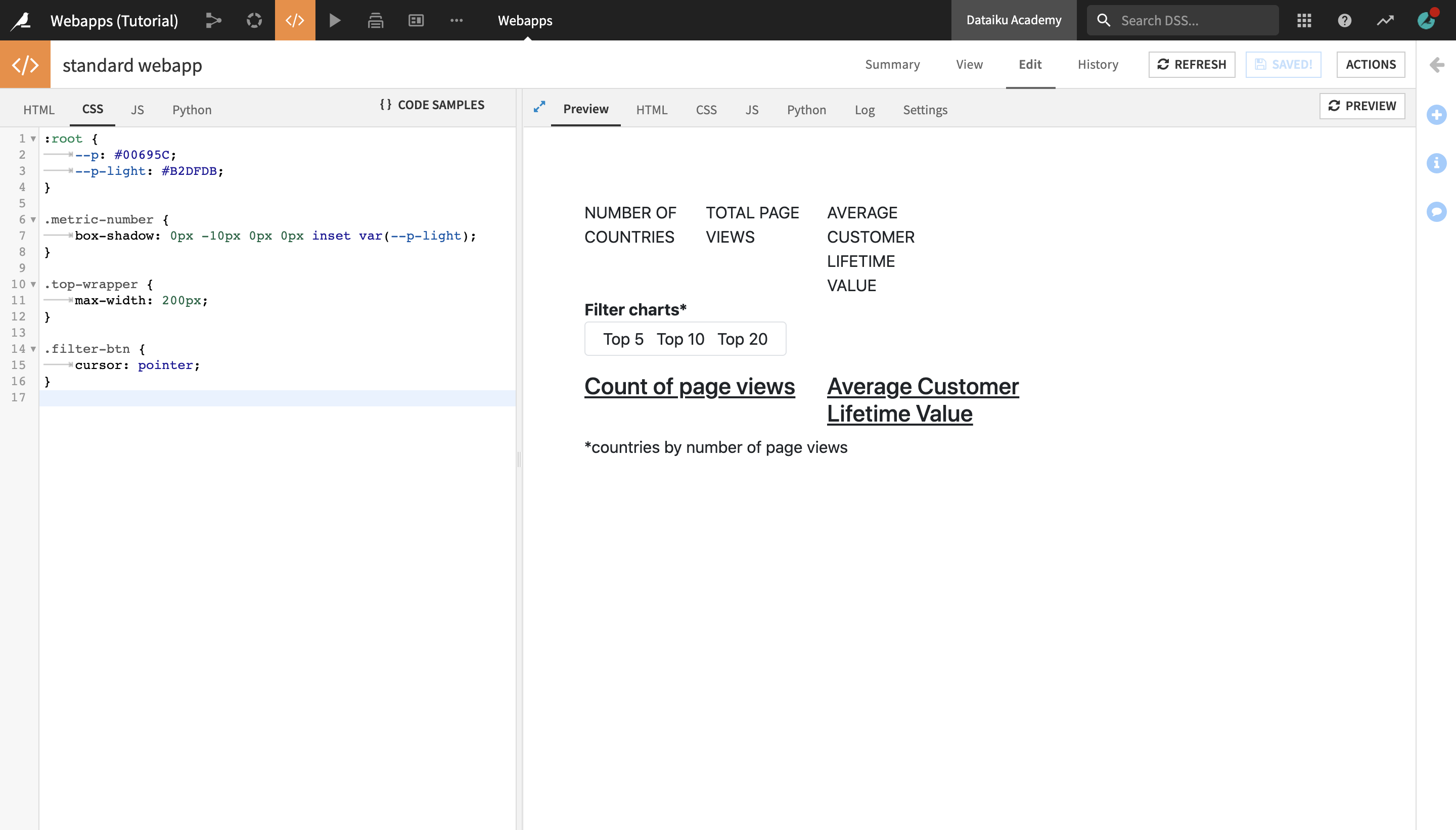
Navigate to the CSS tab of the webapp editor and enter the following code:
:root {
    --p: #00695C;
    --p-light: #B2DFDB;
}

.metric-number {
    box-shadow: 0px -10px 0px 0px inset var(--p-light);
}

.top-wrapper {
    max-width: 200px;
}

.filter-btn {
    cursor: pointer;
}
Note
The :root statement used above is a way to define CSS variables. In this example, we have two variables: “–p” and “–p-light” and they store HEX color codes. We can use such variables in CSS code or in JavaScript, instead of hardcoding them each time.
Click Save.
The Preview tab now displays the app layout with a slightly updated design.
Visualize Metrics and Charts with d3.js
We will now populate the app layout sections with their corresponding metrics and charts.
Navigate to the JS tab of the webapp editor.
Currently, it displays the following block of code, which we defined earlier to retrieve the data from the backend to the frontend and display the dataframe in the log:
$.getJSON(getWebAppBackendUrl('send_data'),function(data){
    data = JSON.parse(data["dataset"]);
    console.log("our data", data);
})
We will now proceed to:
update the three metrics (number of countries, total page views, and average customer lifetime value), by calling the HTML IDs;
update the two graphs based on the user input (“Top 5”, “Top 10” or “Top 20”); and
write functions to draw the two graphs.
Update the Metrics
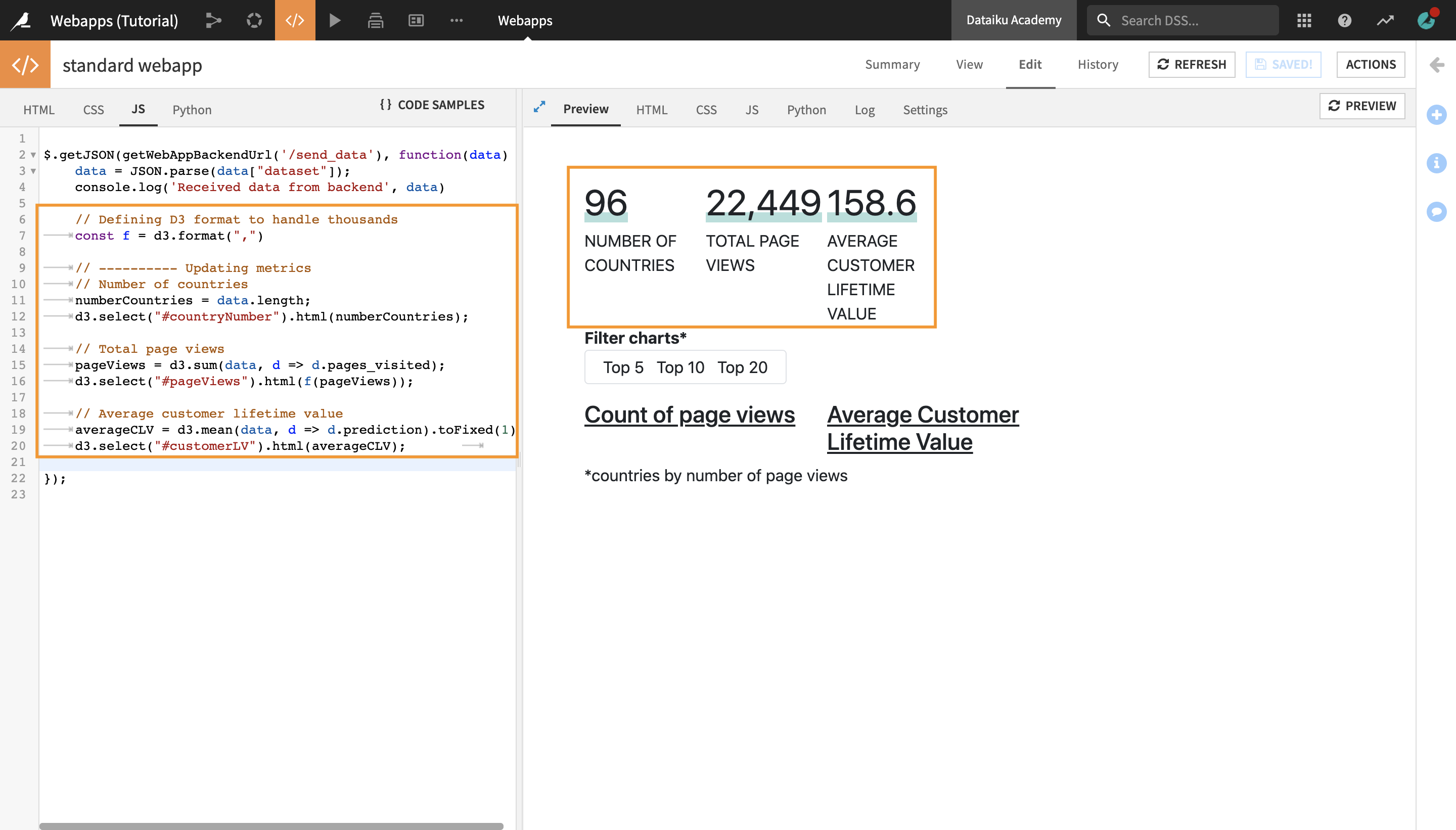
Enter the following code in the JavaScript code editor, just above the two closing brackets at the very end (
})):
// Define D3 format to handle thousands
const f = d3.format(",")

// ---------- Updating metrics
// Number of countries
numberCountries = data.length;
d3.select("#countryNumber").html(numberCountries);

// Total page views
pageViews = d3.sum(data, d => d.pages_visited);
d3.select("#pageViews").html(f(pageViews));

// Average customer lifetime value
averageCLV = d3.mean(data, d => d.prediction).toFixed(1);
d3.select("#customerLV").html(averageCLV);
In the above piece of code:
We defined a constant,
const f = d3.format(",", which helps us format some of the numerical data (e.g.: “1000” will become “1,000”);Then, we updated the HTML code using the
d3.select().html()method, by selecting specific IDs from the HTML page:the number of countries:
data.lengththe number of page views:
d3.sum(data, d => d.pages_visited); andthe mean of the average of Customer Lifetime Value:
d3.mean(data, d => d.prediction).toFixed(1)
Click Save.
The Preview tab now displays the updated metric values.
Update the Graphs Based on User Input
Next, we will set up the graphs so that they update based on user input.
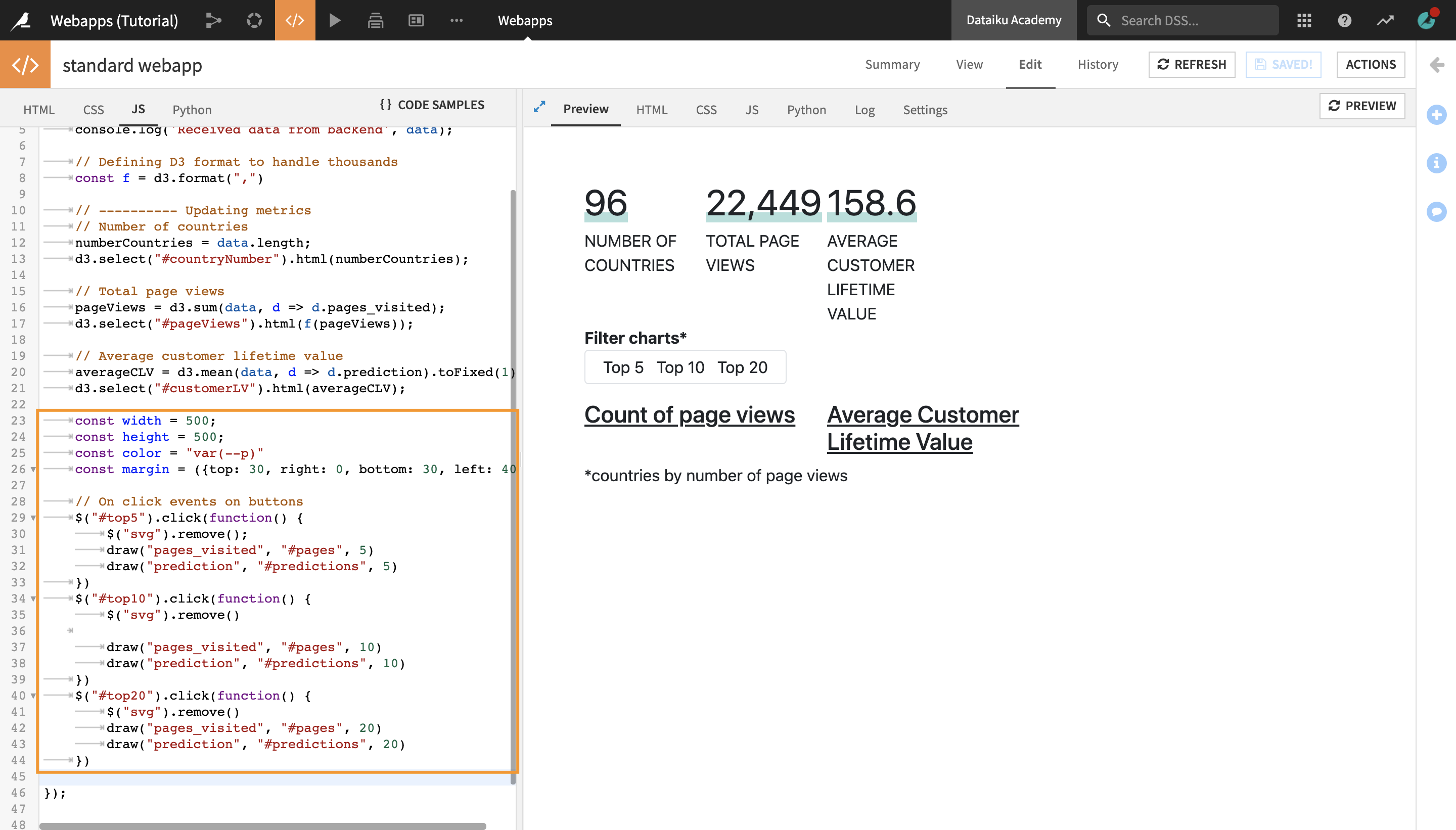
In the below piece of code:
First, we will define four constants in order to set up our SVG graphs. We will use them later on in the code. Notice that the color’s value matches with the CSS variable that we defined in :root;
We will then use jQuery to update the two graphs so that whenever the user clicks on any of the 3 buttons (“Top 5”, “Top 10” and “Top 20”), it will first remove the current SVG elements, and then execute the draw function for both graphs.
Enter the following code in the JavaScript code editor, just above the two closing brackets at the very end (
})):
const width = 500;
const height = 500;
const color = "var(--p)"
const margin = ({top: 30, right: 0, bottom: 30, left: 40})

// On click events on buttons
$("#top5").click(function() {
$("svg").remove();
draw("pages_visited", "#pages", 5)
draw("prediction", "#predictions", 5)
})
$("#top10").click(function() {
$("svg").remove()
draw("pages_visited", "#pages", 10)
draw("prediction", "#predictions", 10)
})
$("#top20").click(function() {
$("svg").remove()
draw("pages_visited", "#pages", 20)
draw("prediction", "#predictions", 20)
        })
Click Save.
Write Functions to Draw the Graphs
Our draw() function will take three inputs:
the appropriate key of our data array (pages_visited or prediction, respectively);
the ID of the appropriate graph (“#pages” or “#predictions” which are defined in the HTML code); and
the number of objects to keep in the data array (5, 10, or 20). Note that our data array is already sorted in the Python code.
Enter the following code in the JavaScript code editor, just above the two closing brackets at the very end (
})):
function draw(val, id, filter) {

    // Reset buttons style and update the button where id matches with filter
    $(".filter-btn").css({"background-color": "#fff","color":"#000","font-weight":"normal"});
    $(`#top${filter}`).css({"background-color": "var(--p-light)","color":"var(--p)","font-weight":"bold"});

    let updatedData = data.slice(0, filter)

    const svg = d3.select(id)
    .append("svg")
    .attr("viewBox", [0, 0, width, height]);


    let x = d3.scaleBand()
    .domain(d3.range(updatedData.length))
    .range([margin.left, width - margin.right])
    .padding(0.1)

    let y = d3.scaleLinear()
    .domain([0, d3.max(updatedData, d => d[val])]).nice()
    .range([height - margin.bottom, margin.top])

    let xAxis = g => g
    .attr("transform", `translate(0,${height - margin.bottom})`)
    .call(d3.axisBottom(x).tickFormat(i => updatedData[i].ip_country_code).tickSizeOuter(0))

    let yAxis = g => g
    .attr("transform", `translate(${margin.left},0)`)
    .call(d3.axisLeft(y).ticks(null, updatedData.format))
    .call(g => g.select(".domain").remove())
    .call(g => g.append("text")
        .attr("x", -margin.left)
        .attr("y", 10)
        .attr("fill", "currentColor")
        .attr("text-anchor", "start")
        .text(updatedData.y))

    svg.append("g")
        .attr("fill", color)
        .selectAll("rect")
        .data(updatedData)
        .join("rect")
        .attr("x", (d, i) => x(i))
        .attr("y", d => y(0))
        .attr("height", 0)
        .attr("width", x.bandwidth())
        .transition()
        .duration(2000)
        .attr("y", d => y(d[val]))
        .attr("height", d => y(0) - y(d[val]))

    svg.append("g")
        .call(xAxis);

    svg.append("g")
        .call(yAxis);
    }

    // Set default input values
    draw("pages_visited", "#pages",10);
    draw("prediction", "#predictions",10);
Click Save.
The updated Preview tab now displays the finished state of the webapp.
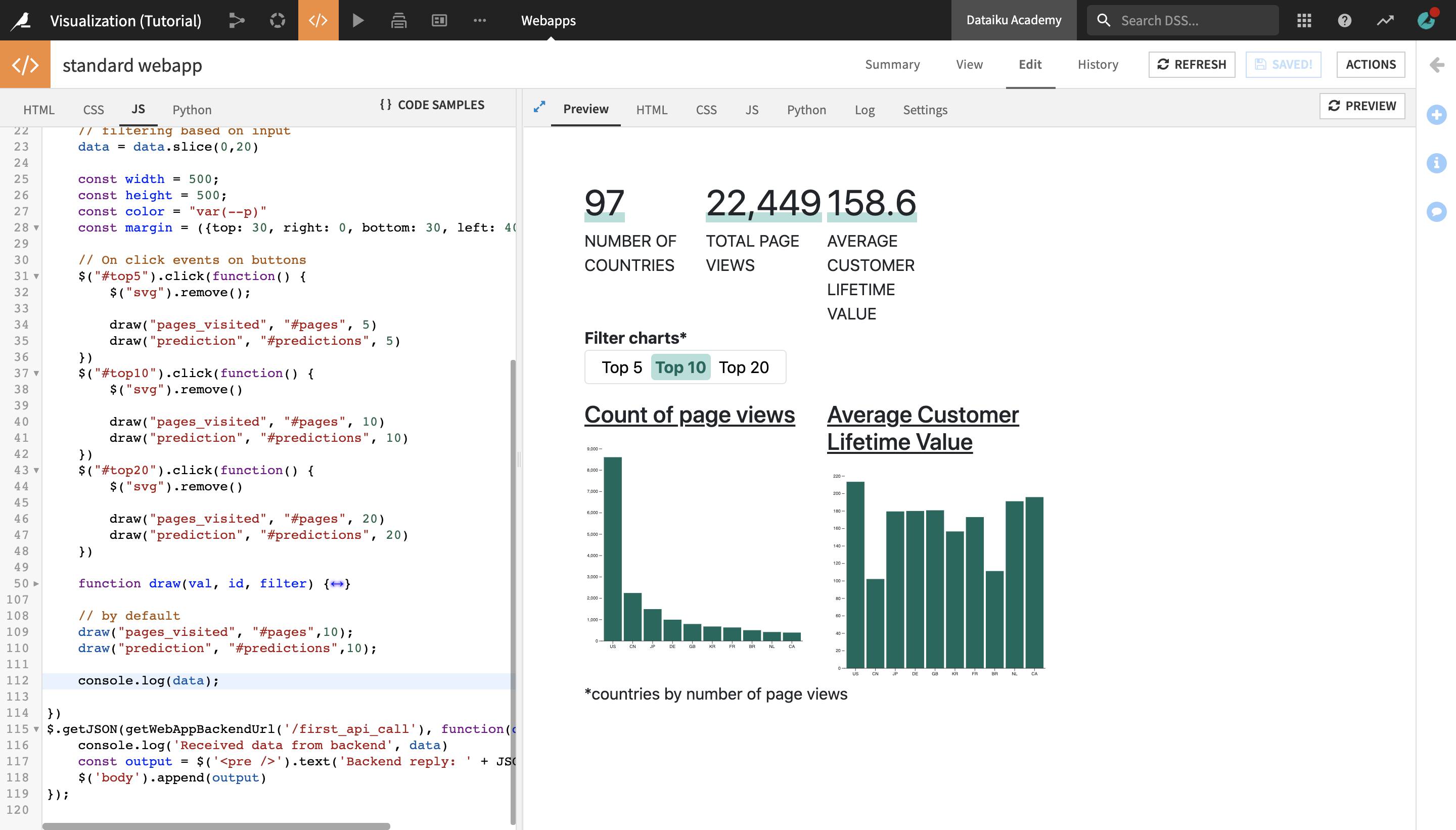
In the code above:
Using jQuery, we added some styling to the newly clicked button;
We updated the array based on the filter variable;
We created an SVG element (
const svg = d3.select(id))to then add various elements to it (rectangle shapes for the bar charts, X and Y axis, etc.);We created scales: (using
d3.scaleBand()andd3.scaleLinear());We created the X axis and Y axis;
- We appended the bars:
so that they use the
rectshape;with the
transition()d3.js method in order to animate their movement; andwe called the axis with
call(xAxis)andcall(yAxis);
Finally, we called the draw function for the two graphs in order to set them to display the “Top 10” countries by default.
You can test your webapp’s interactivity by changing the number of countries to display from the Filter charts section. To do this:
Navigate to the View tab to view your finished webapp.
Click the Top 20 button in the Filter charts section.
Observe as the values of the metrics and charts change.
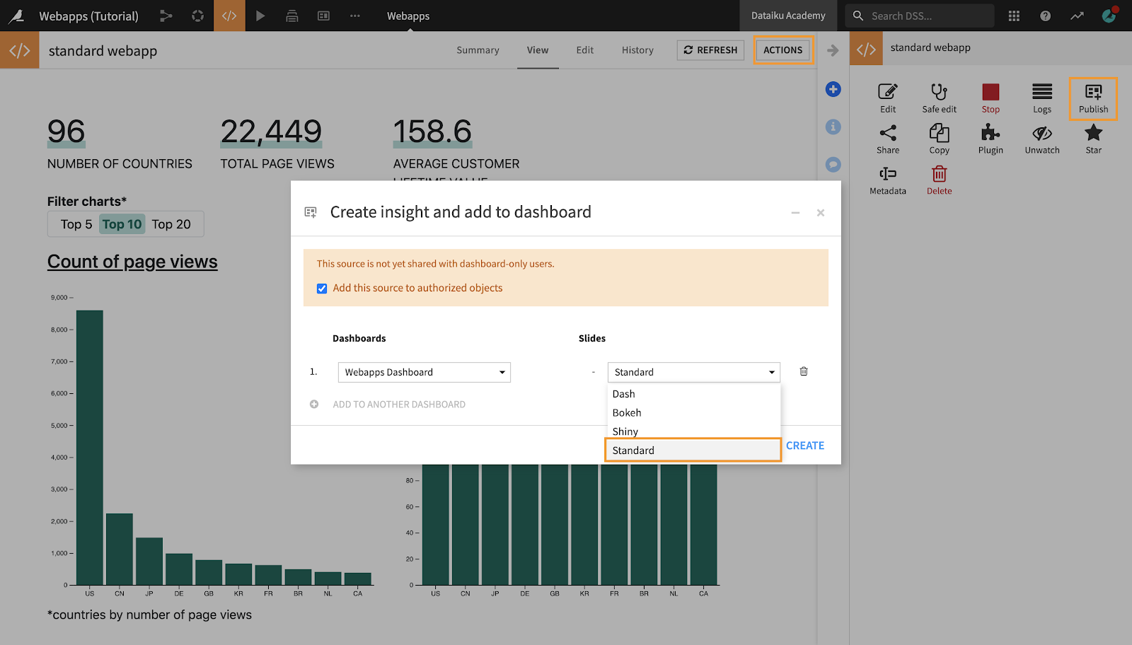
Publish the Webapp on a Dashboard
When you are done with editing, you can publish your webapp on a dashboard.
Click Actions in the top-right corner of the screen.
From the Actions menu, click Publish.
Select the dashboard and slide you wish to publish your webapp on.
Click Create.
You are navigated to the Edit tab of the dashboard.
Note
In the Edit tab of a dashboard, you can edit the way your webapp appears, or add other webapps, as well as other types of insights.
Optionally, you can drag and resize your webapp, or change its title and display options from the Tile sidebar menu. Click Save when you’re done.
Click View to see how your webapp is displayed on the dashboard.
What’s Next
Using Dataiku DSS, you have created an interactive Dash webapp and published it to a dashboard.
To continue learning about webapps, you can:
take another tutorial on using Standard webapps in Dataiku DSS;
browse articles in the Webapps section of the Dataiku Knowledge base.