Concept: Handling Text Features for ML

At this point, we have applied some basic text cleaning steps to our dataset and created a few simple numeric features. We are ready to create features for training a model, in this case, one to classify spam and non-spam (ham) emails.

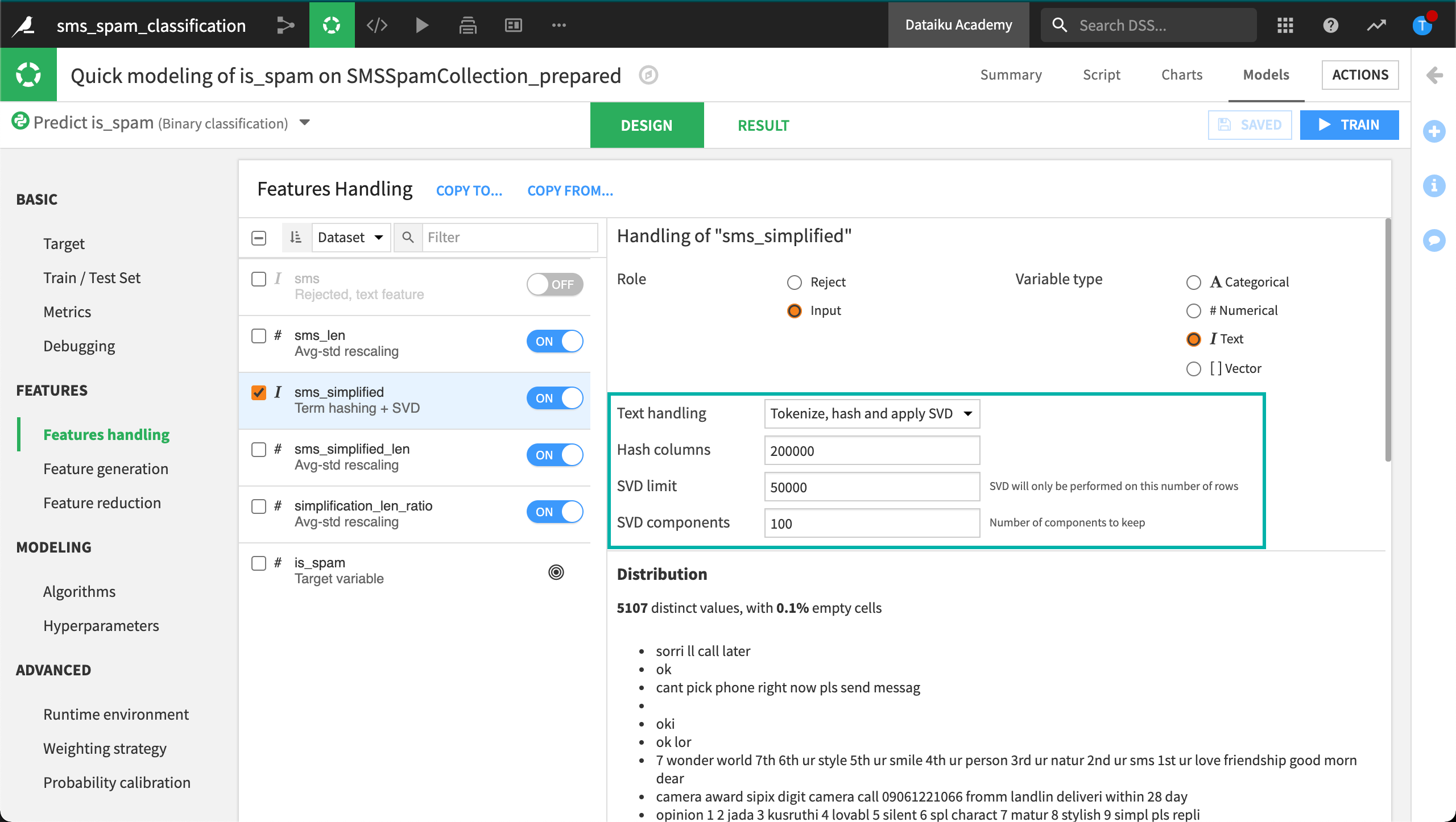
Before feeding this data to machine learning algorithms, however, we have to decide how Dataiku DSS should handle the text when it computes the features. This is done in the Features handling pane of a model’s Design tab.

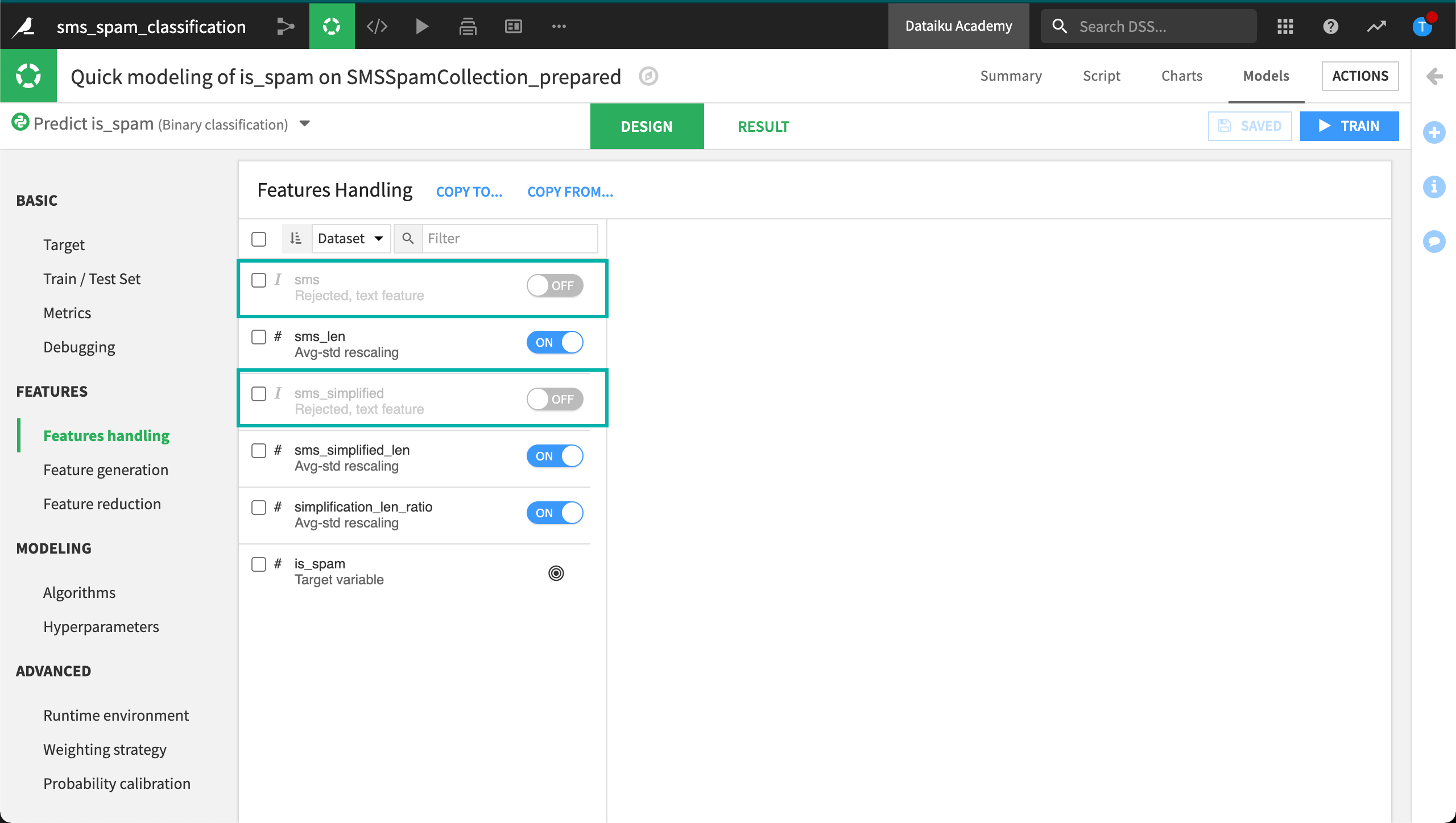
Here, we can see that Dataiku DSS has rejected the two text columns as features for the model. Dataiku DSS rejects text columns as features by default because text is more expensive in terms of memory processing. To add these columns as features, we must manually select them.

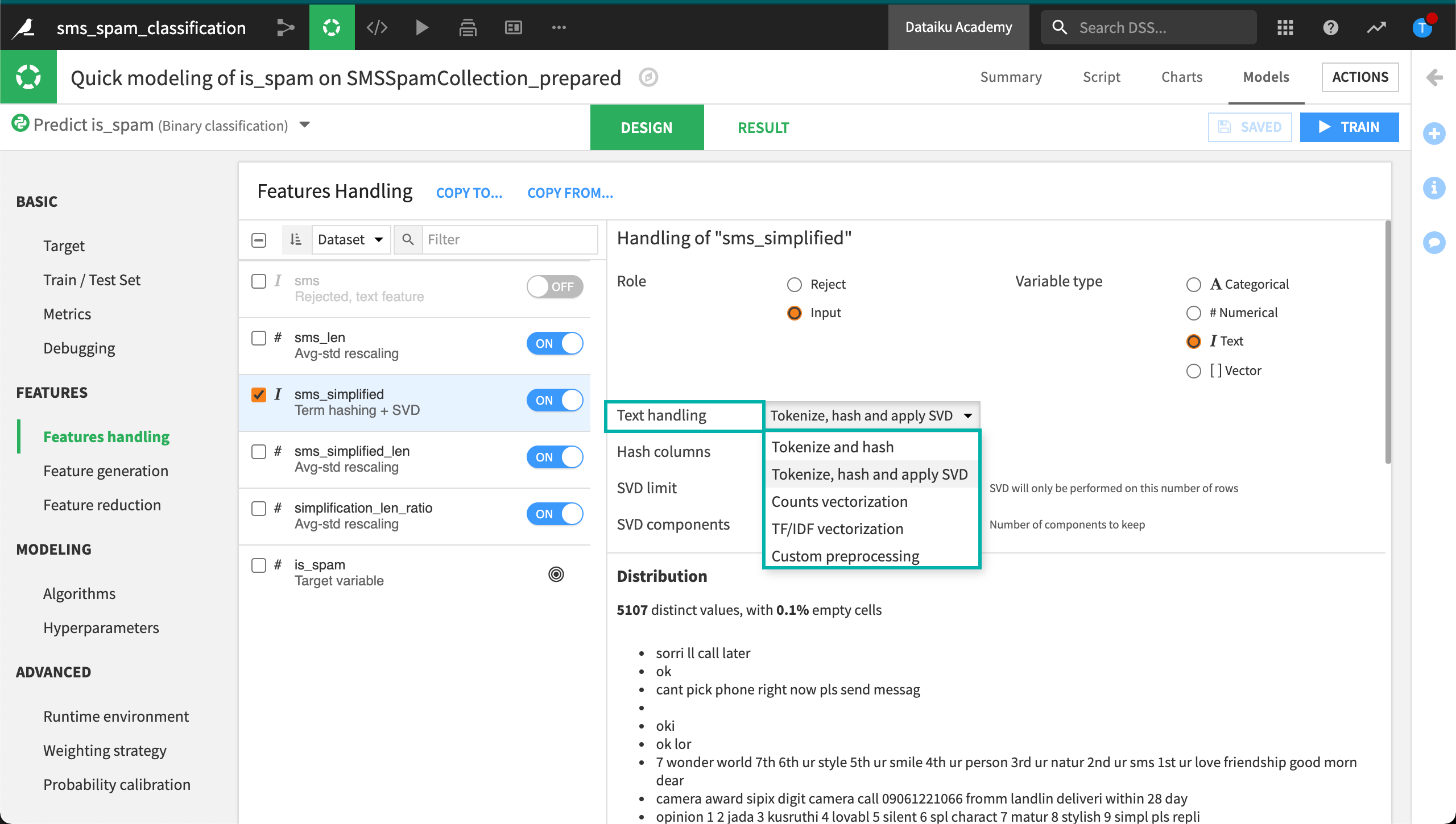
For any text feature, Dataiku DSS can handle it in one of five ways:

• Term hashing

• Term hashing + SVD

• Count vectorization

• TF-IDF vectorization

• Custom preprocessing

To learn more about custom preprocessing, visit the Academy course, Custom ML Models.

Term Hashing (Tokenize and hash)

To understand the first method term hashing, or “Tokenize and hash”, let’s return to our example of encoding categorical values, such as colors, into numeric features.

Term hashing is a similar method to one-hot encoding, except it outputs hashes to represent each unique word of the text.

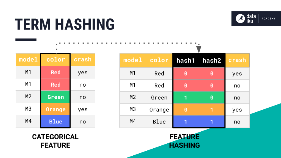
Together, these two columns of zeros and ones are able to represent the four unique colors. But imagine how many columns we would need if we had thousands of unique words!

The dimensionality of the training dataset would be huge, creating major computational headaches. Also, notice that no individual hash column on its own represents a single color, or in our case, word, and so the model will be more difficult to interpret.

When we try applying the “Tokenize and hash” method, Dataiku DSS warns us that this method will create an extremely large number of sparse columns. As warned, we find that the random forest model fails to complete training. We ran out of memory.

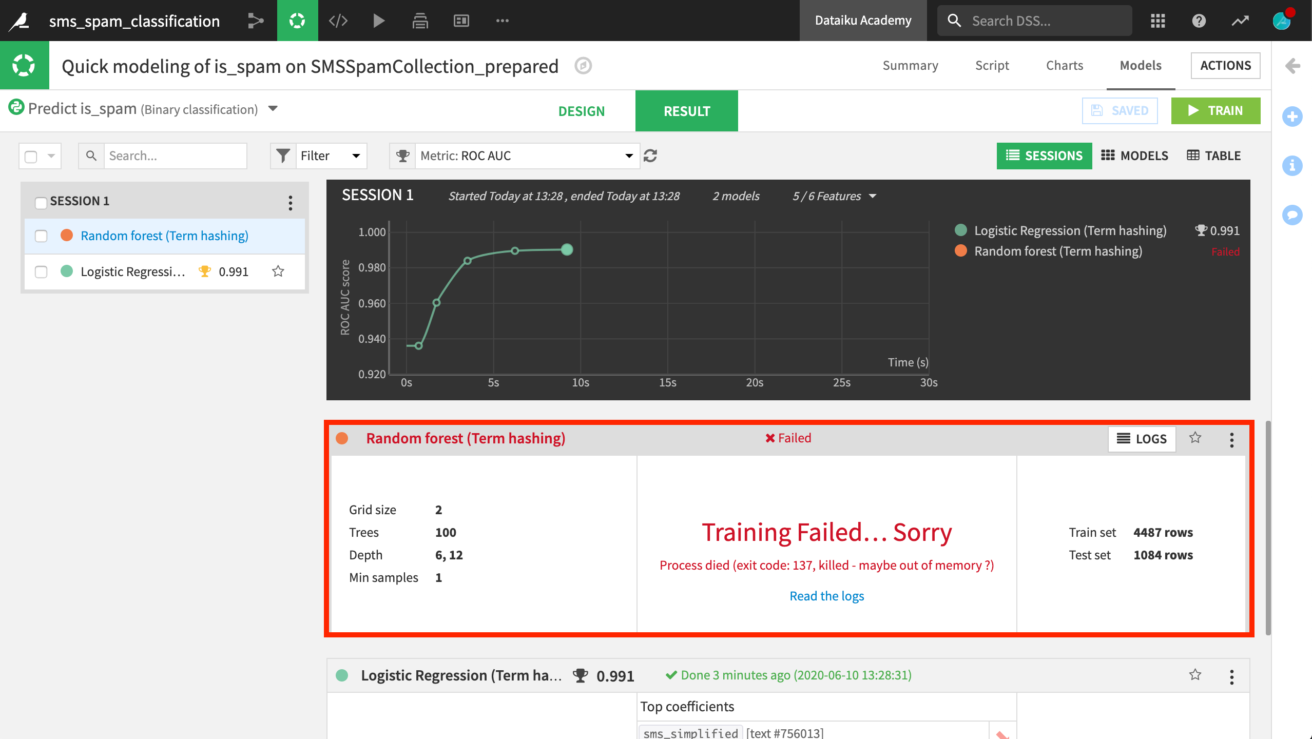
The logistic regression model, however, performed excellently. As this is just a toy dataset, the performance of all models we will build will be very high.

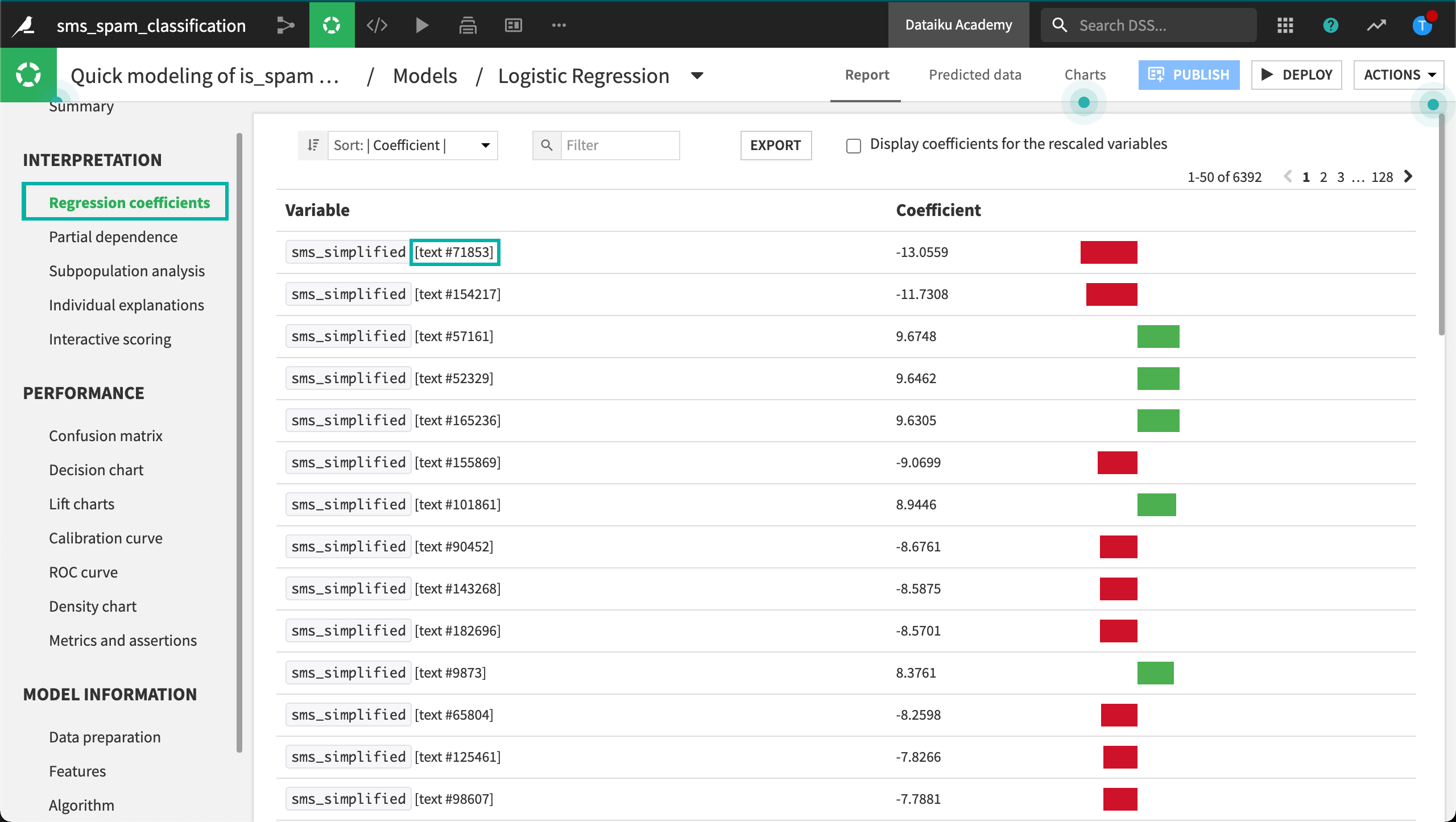
Let’s look at the features. On closer inspection, we can see that this logistic regression model trained on over 1 million features!

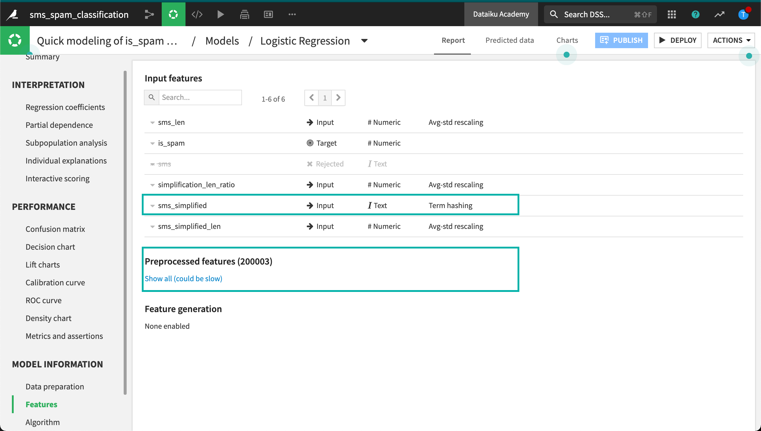
If we look at the regression coefficients, it is not possible to interpret these features as they don’t actually represent individual words.

Term Hashing + SVD (Tokenize, hash and apply SVD)

Let’s first solve the computational problem encountered by the term hashing method by applying a dimensionality reduction method called SVD, or Singular Value Decomposition. We won’t go into the mathematics behind SVD–only how to configure it in Dataiku DSS.

Increasing the number of hash columns or the SVD limit will increase the accuracy of the model, but it will take longer to train. The last field, SVD components, specifies the final number of features to be created.

When using the SVD method, we no longer have a memory error when training the random forest model. Although this method is generally the least accurate and least interpretable, it is the most scalable option. This is why it is the default selection in Dataiku DSS.

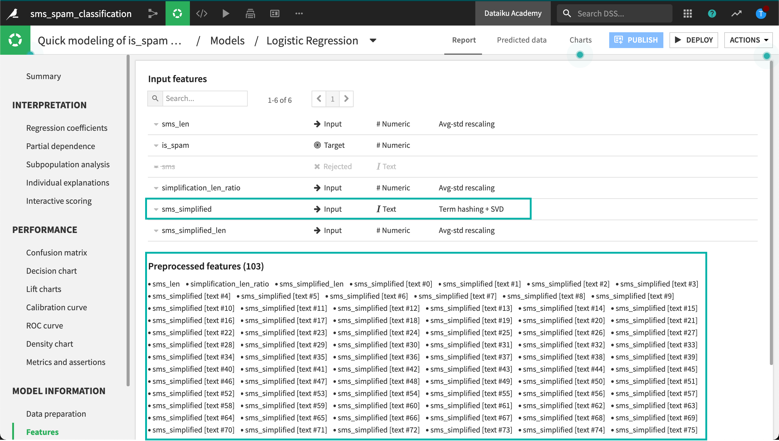
Again, performance is excellent, but focus on the features. Now the model only has 103 preprocessed features, 3 numeric and 100 SVD components.

Count Vectorization

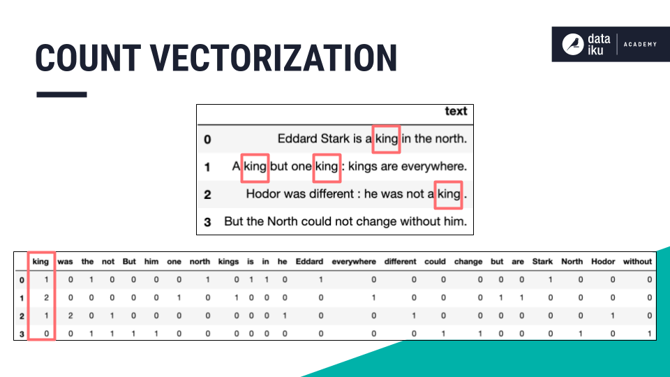
SVD has solved our computational problem, but how should we interpret hash columns like “sms_simplified [text #0]” or “sms_simplified [text #1]”? We can solve this problem by going back to the bag of words approach.

When applying count vectorization, think of creating an occurrence matrix for each word in the text column.

Dataiku DSS allows us to easily implement this approach. There are a few helpful settings we should consider.

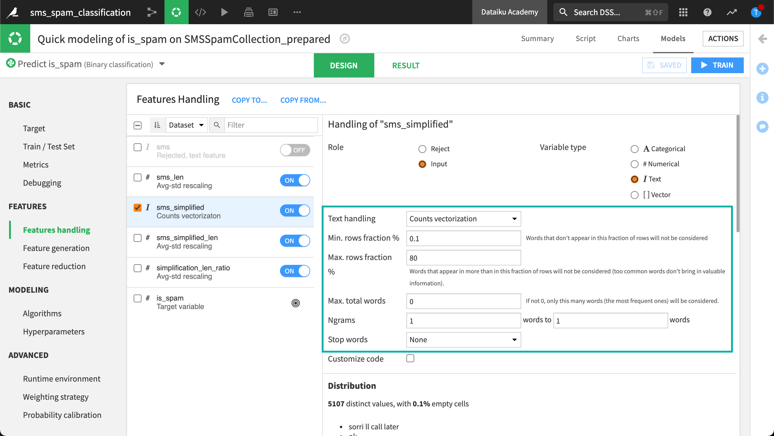
The first field, Min. rows fraction %, can be used to filter out words that do not appear in a certain minimum percentage of rows. This can help reduce dimensionality by removing uncommon words.

The second field, Max. rows fraction %, achieves the opposite. Just like very uncommon words, extremely common words are unlikely to contain predictive information, and so can be filtered out.

We can also define what kind of N-grams to include. For example, do we only want 1-grams? Or do we also want to create 2-grams?

We have already removed stopwords using the Prepare recipe so we do not need to do that here.

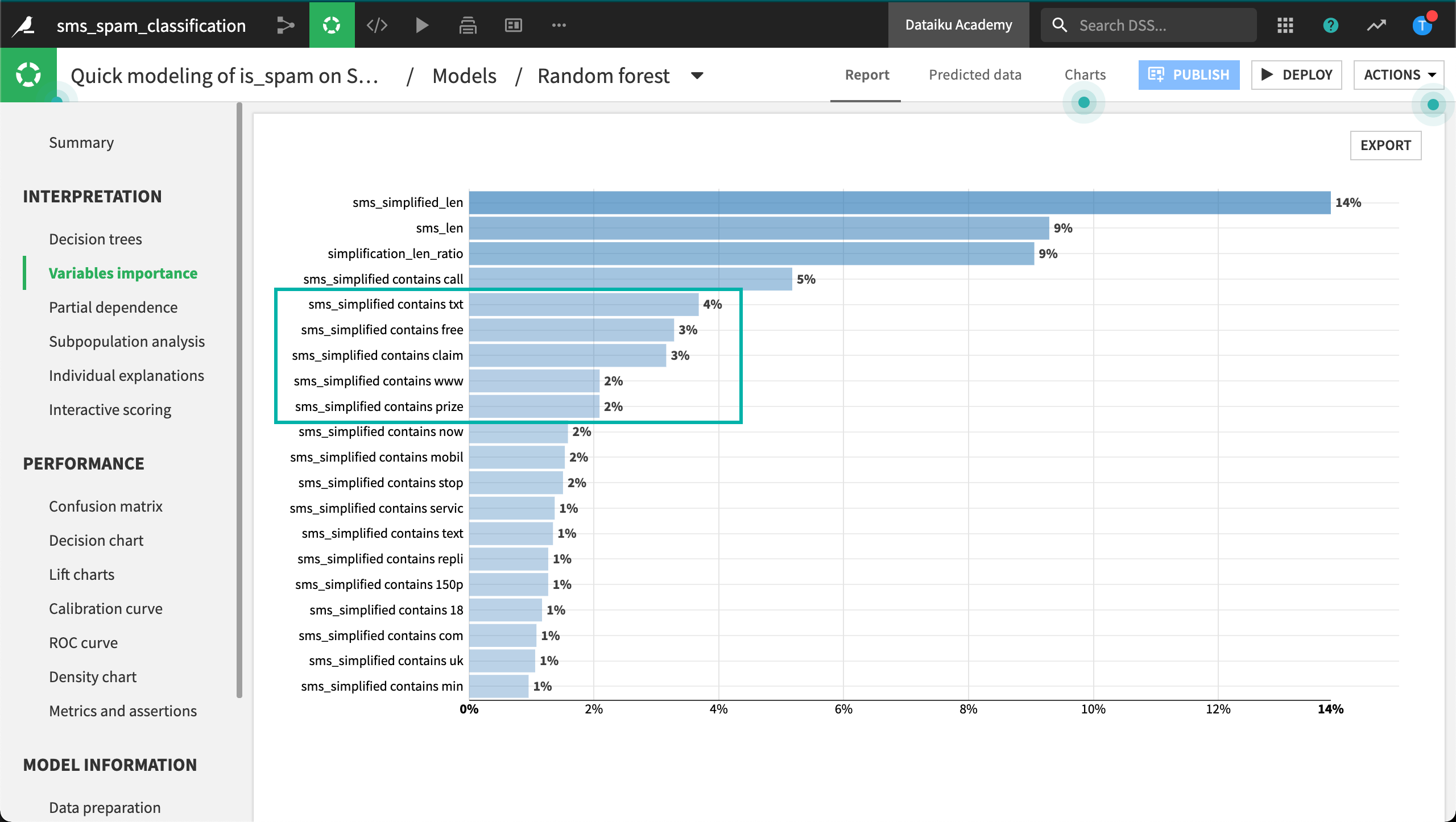
When these models finish training, we can see a difference in interpretability. Aside from the numeric features, having the word ‘call’, ‘txt’, or ‘claim’ in the message is associated with spam. That sounds reasonable!

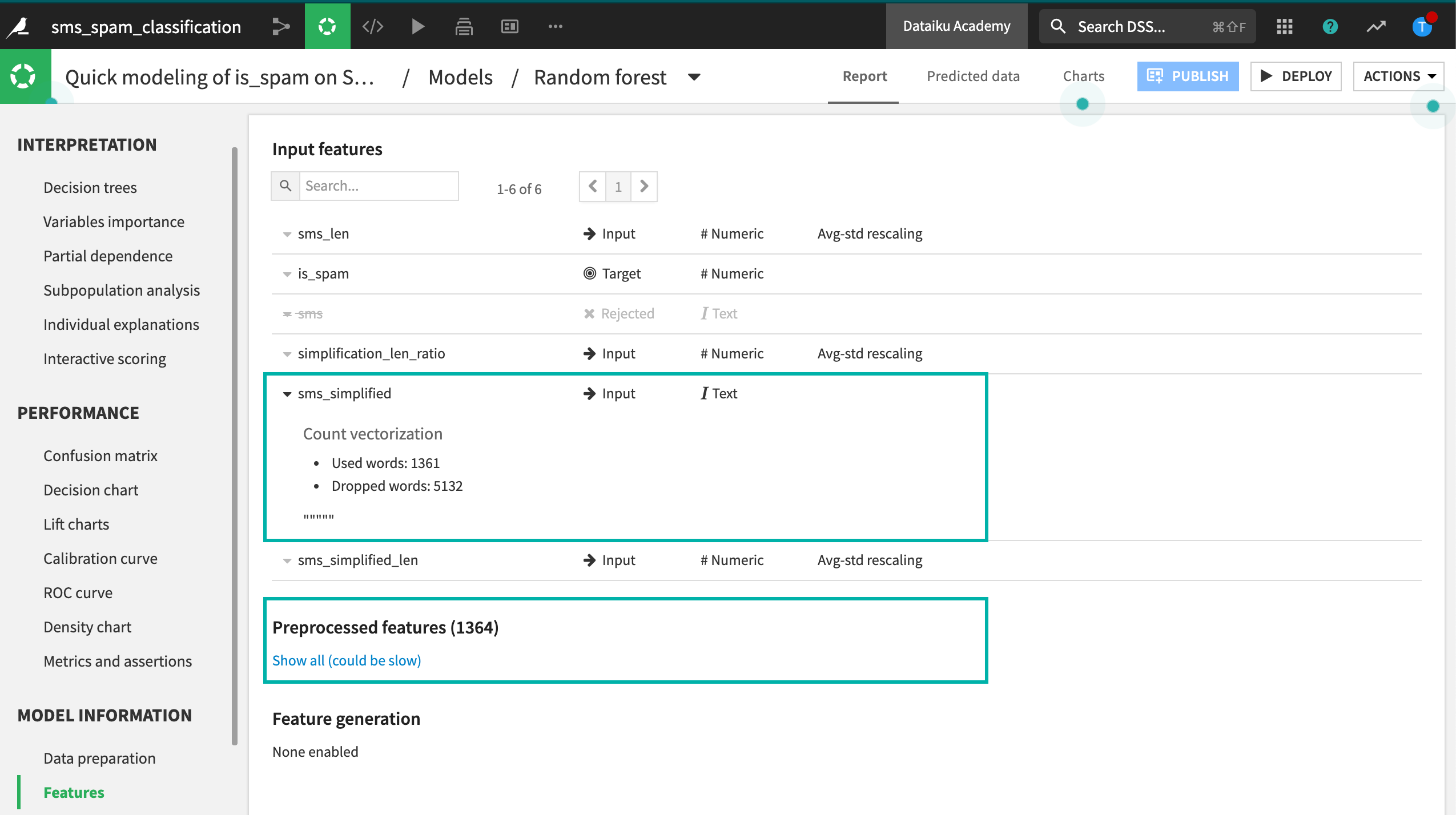
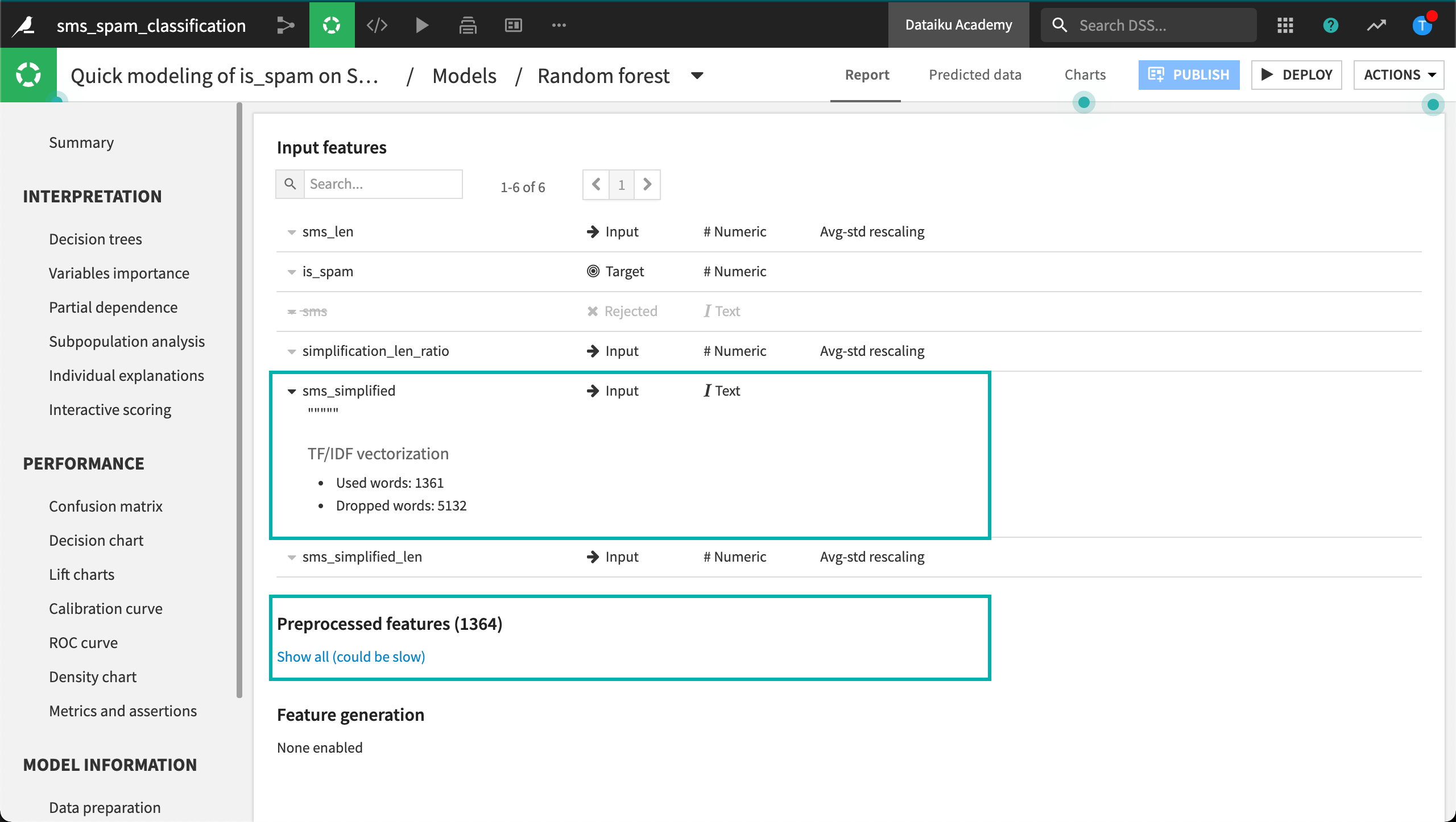
Let’s look closer at the features. We can see which words the model has used and which it has dropped. These will vary according to the settings in the design.

TF-IDF Vectorization

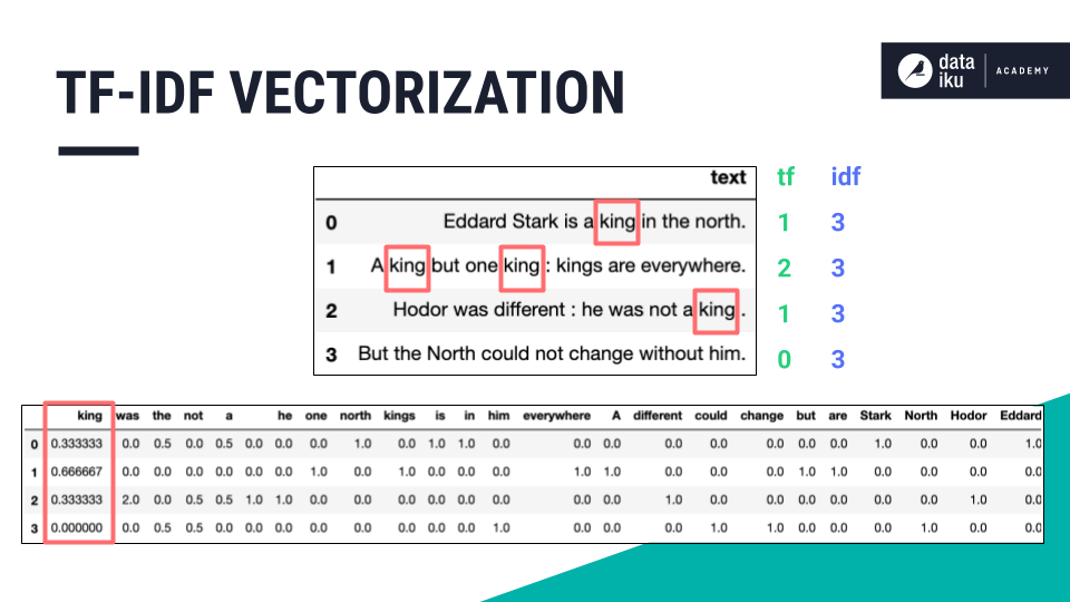
Similar to count vectorization, one last text handling option is TF-IDF vectorization.

Term frequency - inverse document frequency scales word occurrences by the inverse of their frequencies in the entire dataset instead of building the occurrence matrix on counts alone.

When selecting this option in Dataiku DSS, all of the settings for establishing minimum and maximum thresholds are the same as count vectorization. This time let’s also include 2-grams as potential features.

Looking at the results, we can see which words were influential in classifying spam just as we could when using counts vectorization. But with TF-IDF vectorization, we also see the IDF score of each text feature.

We can also note that including 2-grams in this case does not seem to have been worth the cost. The model did include a few hundred 2-grams as features, but thousands more were dropped based on the feature handling parameters– without any improvement in accuracy.

What’s next?

Now having built models with four different text handling strategies, we can begin to see some of the strengths and weaknesses of each text handling strategy and compare the scalability and interpretability of each method.

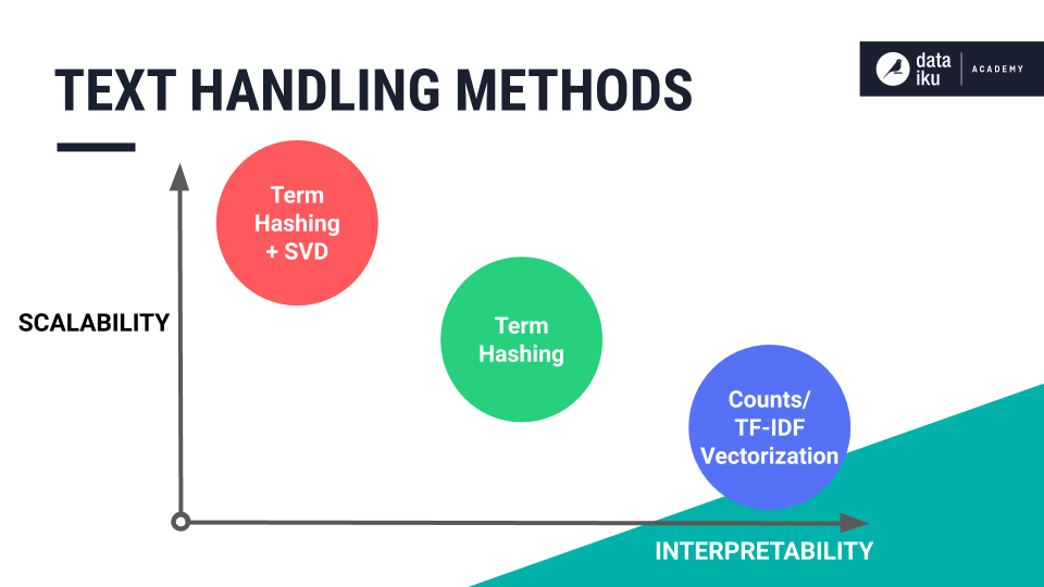
You can try out these strategies for yourself in the next hands-on lesson!