Predictive Maintenance

Overview

Business Case

We are part of a data team working on a predictive maintenance use case at a car rental company.

Unexpected problems on the road for a rental car can really add to costs because of the associated repairs, unavailability, and the inconvenience to customers. With this in mind, the company wants to replace those cars that are more likely to break down before a problem occurs, thereby minimizing the chance of a rental car breaking down on a customer. At the same time, replacing otherwise healthy vehicles too often would not be cost-effective either.

The company has some information on past failures, as well as on car usage and maintenance. As the data team, we are here to offer a data-driven approach. More specifically, we want to use the information we have to answer the following questions:

• What are the most common factors behind these failures?

• Which cars are most likely to fail?

These questions are interrelated. As a data team, we are looking to isolate and understand which factors can help predict a higher probability of vehicle failure. To do so, we’ll build end-to-end predictive models in Dataiku DSS. We’ll see an entire advanced analytics workflow from start to finish. Hopefully, its results will end up as a data product that promotes customer safety and has a direct impact on the company’s bottom line!

Supporting Data

We’ll need three datasets in this tutorial. Find their descriptions and links to download below:

• usage: number of miles the cars have been driven, collected at various points

• maintenance: records of when cars were serviced, which parts were serviced, the reason for service, and the quantity of parts replaced during maintenance

• failure: whether a vehicle had a recorded failure (not all cases are labelled)

An Asset ID, available in each file, uniquely identifies each car. Some datasets are organized at the vehicle level; others are not. A bit of data detective work might be required!

Workflow Overview

By the end of this walkthrough, your workflow in Dataiku DSS should mirror the one below. Moreover, the completed project can be found in the Dataiku gallery.

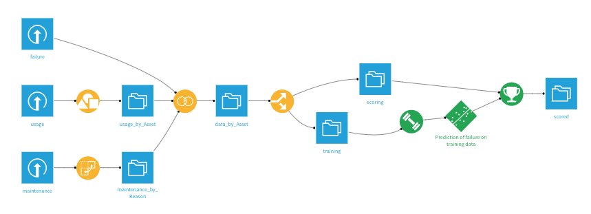
In order to achieve this workflow, we will complete the following high-level steps:

• Import the data

• Clean, restructure and merge the input datasets together

• Split the merged dataset by whether outcomes are known and unknown, i.e., labelled and unlabelled

• Train and analyze a predictive model on the known cases

• Score the unlabelled cases using the predictive model

Prerequisites

You should be familiar with:

• The Basics courses

• Machine learning in Dataiku DSS

Technical Requirements

To complete this walkthrough, the following requirements need to be met:

• Have access to a Dataiku DSS instance–that’s it!

Creating the Project and Importing Datasets

First, we will import into Dataiku DSS the three input files found in the Supporting Data section of the previous lesson. Detailed import steps are provided below. If comfortable importing flat files, feel free to skip to the Preparing the Usage Dataset lesson.

Note

Workflows are organized as projects on a DSS instance. The project home page contains metadata (description, tags), records of activities, and much more.

1. From the Dataiku homepage, go to + New Project > Blank Project. Name it Predictive Maintenance. Note that the new project is automatically assigned a project key. We can leave the default or assign something else in its place, but it cannot be changed once the project is created.

2. Let’s create the first dataset and name it usage. Here’s one method to do that:

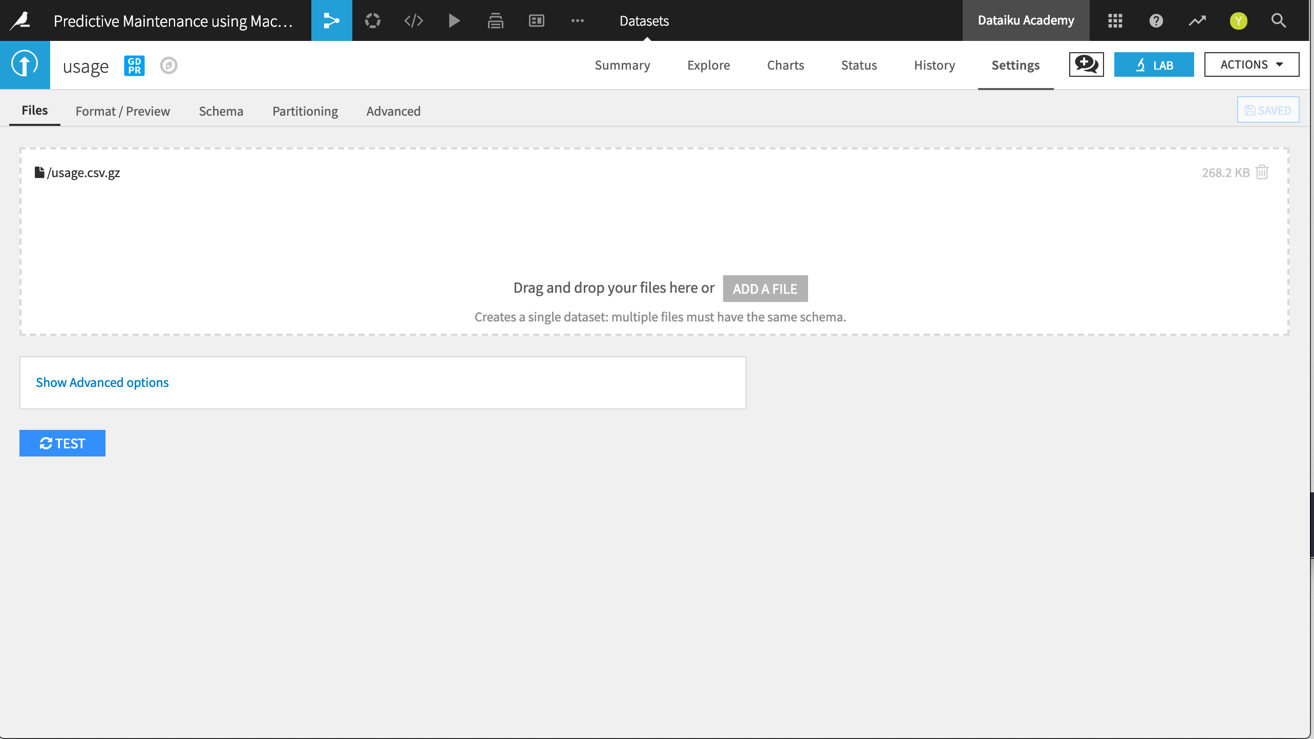
• Click on the + Import Your First Dataset button on the project homepage.

• Select Files > Upload your files.

• Upload the usage.csv.gz file downloaded from the Supporting Data section of the previous lesson.

• Click on Preview to view the default import settings used by Dataiku DSS.

  • These settings can be adjusted as necessary. For example, if the data is stored in a JSON format, then we can detect that in this step.

• If the import settings look ok, click Create.

3. Repeat these actions to import the two remaining files as datasets: failure.csv.gz and maintenance.gz.csv.

Once all three datasets are present in the Flow, you are ready to proceed.

Preparing the Usage Dataset

The usage dataset tracks the mileage for rental cars, identified by their Asset ID, at a given point in Time.

• The Use variable records the total number of miles a car has driven at the specified Time.

• The units of the Time variable are not clear. Perhaps days from a particular date? This might be a question for the data engineers who produced this dataset.

• Here Asset ID is not unique, i.e., the same rental car might have more than a single row of data.

On importing the CSV file, from the Explore tab, we can see that the columns are stored simply as “string” type (the grey text beneath the column header), even though Dataiku DSS can interpret the meanings to be “text”, “integer”, and “decimal” (the blue text beneath the storage type).

Note

For more information, please see the reference documentation expounding on the distinction between storage types and meanings.

Accordingly, with data stored as strings, we won’t be able to perform any mathematical operations on seemingly-numeric columns such as Use. Let’s fix this.

1. Navigate to the Settings > Schema tab, which shows the storage types and meanings for all columns.

2. Click Check Now to determine that the schema and data are consistent.

3. Then click Infer Types from Data to allow DSS to assign new storage types and high-level classifications.

Returning to the Explore tab, note that although the meanings (written in blue) have not changed, the storage types in grey have updated to “string”, “bigint”, and “double”.

Note

As noted in the UI, this action only takes into account the current sample, and so should be used cautiously. There are a number of different ways to perform type inference in Dataiku DSS, each with their own pros and cons, depending on your objectives. The act of initiating a Prepare recipe, for example, is another way to instruct DSS to perform type inference.

For most individual cars, we have many Use readings at many different times. However, we want the data to reflect the individual car so that we can model outcomes at the vehicle-level. Now with the correct storage types in place, we can perform the aggregation with a visual recipe:

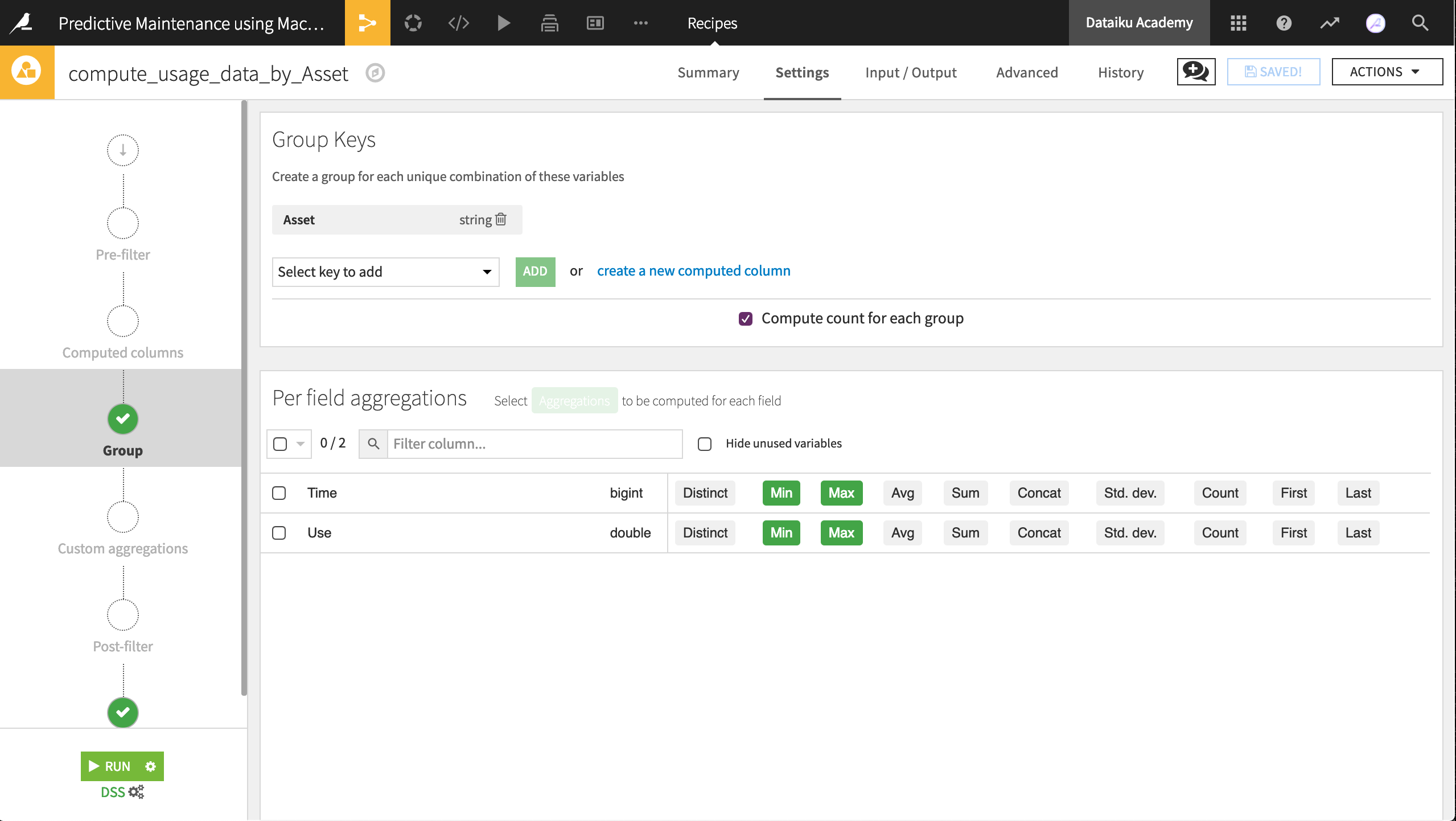
1. From the usage dataset, initiate a Group By recipe from the Actions menu.

2. Choose to Group By Asset in the dropdown menu.

3. Keep the default output dataset name usage_by_Asset.

4. In the Group step, we want the count for each group (selected by default). Add to this the Min and Max for both Time and Use.

5. Run the recipe, updating the schema to six output columns.

Now aggregated at the level of a unique rental car, the output dataset is fit for our purposes. Let’s see if the maintenance dataset can be brought to the same level.

Preparing the Maintenance Dataset

The maintenance dataset documents activity that has occurred with respect to a given Asset, organized by Part (what was repaired) and Time (when it was repaired). A Reason variable codifies the nature of the problem.

As we did for the usage dataset, we want to organize the maintenance dataset to the level of unique vehicles. For the usage dataset, we achieved this with the Group recipe. Here, we’ll use the Pivot recipe.

While the current dataset has many observations for each vehicle, we need the output dataset to be “pivoted” at the level of each vehicle; that is, transformed from narrow to wide.

Note

Data transformation from narrow to wide is a common step in data preparation. Different statistical software packages and programming languages have their own terms to describe this transformation. Wide and narrow is one standard, but there are of course others.

1. As done for the usage dataset, infer storage types so that the variables Time and Quantity are no longer stored as strings.

2. Next, use the Pivot recipe to restructure the dataset at the level of each vehicle. In detail:

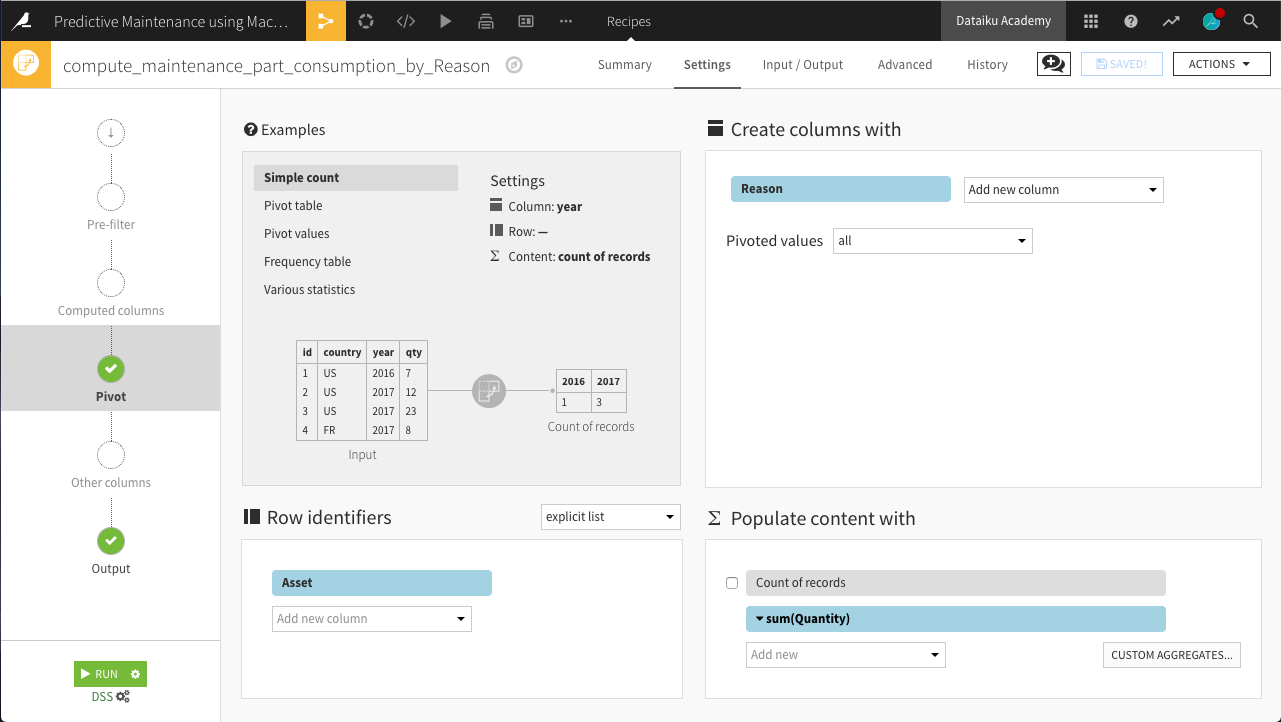
• With maintenance chosen as the input dataset, choose to Pivot By Reason.

• Keep the default output dataset name maintenance_by_Reason and Create Recipe.

• At the Pivot step, select Asset as the row identifier.

• Reason should already be selected under Create columns with. Although it should make no difference in this case, change Pivoted values to all so that all values of Reason are pivoted into columns.

• Populate content with the sum of Quantity. Deselect Count of records.

3. Run the recipe.

Note

More detailed information on the Pivot recipe can be found in the reference documentation or the Visual Recipes Overview.

Preparing the Failure Dataset

The Failure dataset has only two columns: Asset ID and failure_bin.

• Here Asset IDs are unique (i.e., one row for each ID), so we are already structured at the level of individual cars. The Analyze tool is one quick method to verify this important property.

• The failure_bin variable contains 0’s and 1’s representing failures of the associated Asset. We can use this variable as a label to model predictions for failures among the fleet.

Only one preparation step is needed here. As done with the previous two datasets, use the Infer Types from Data from within the Settings > Schema tab so that failure_bin is stored as a bigint.

Our workflow is now beginning to look like a data pipeline. Next we’ll merge all of our datasets together!

Merging the Datasets

We now have three datasets at the same level of granularity: the Asset, i.e., an individual rental car. Joining them together will give us the most possible information for a model. With the same Asset ID in each dataset, we can easily join the datasets with a visual recipe.

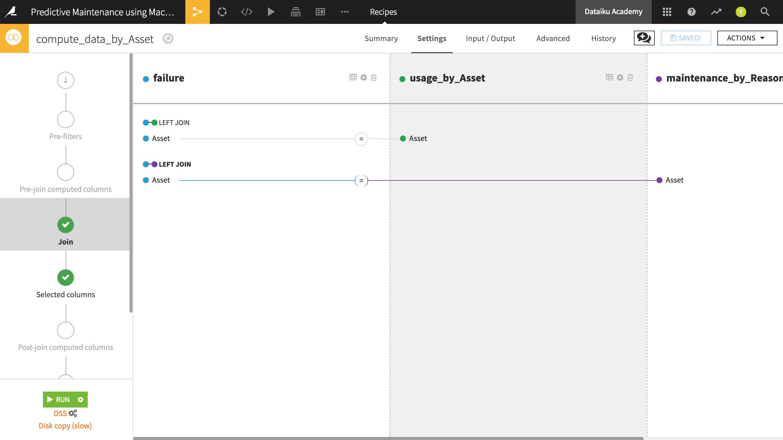
1. From the failure dataset, initiate a Join recipe.

2. Add usage_by_Asset as the second input dataset.

3. Name the output data_by_Asset. Click Create Recipe.

4. Add maintenance_by_Reason as the third input dataset.

5. Both joins should be Left Joins. Asset should be the joining key in all cases.

6. Run the recipe and update the schema to 21 columns.

Note

Check the reference documentation for more information on the Join recipe.

data_by_Asset now holds information from maintenance and usage, labelled by failures. Congratulations, great work!

Creating the Training & Scoring Datasets

To train models, we’ll use the Split recipe to create two separate datasets from the merged dataset, data_by_Asset:

• a training dataset will contain labels for whether or not there was a failure event on an asset. We’ll use it to train a predictive model.

• a scoring dataset will contain no data on failures, i.e., unlabelled, so we’ll use it to predict whether or not these assets have a high probability of failure.

Here are the detailed steps:

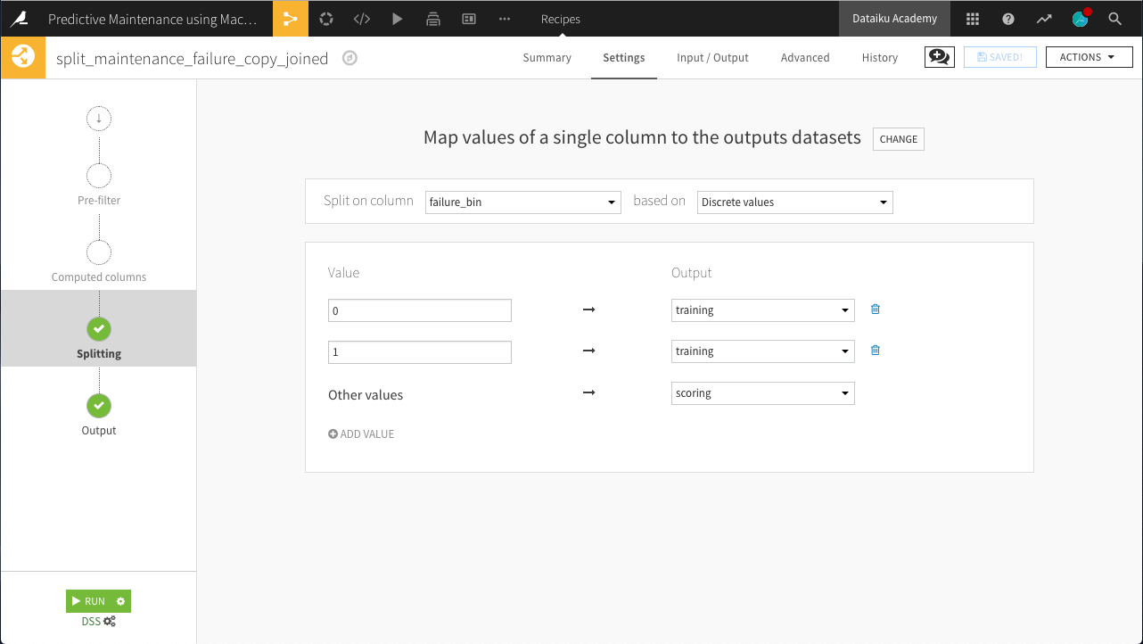
1. From the data_by_Asset dataset, initiate a Split recipe.

2. Add two output datasets, named training and scoring, selecting Create Dataset each time. Then Create Recipe.

3. At the Splitting step, choose to Map values of a single column. Then choose failure_bin as the column on which to split.

4. Assign values of 0 and 1 to the training set, and all “Other values” to the scoring set. (From the Analyze tool, we can see that these are the only possible values).

5. Run the recipe.

Note

In this example data, it is unclear exactly why the unlabelled data used for the scoring data are missing. Are they missing at random? Or do they represent a population that is different in some meaningful way from the labelled data now in the training dataset? This is an important data science question, but not one we can answer without knowing more about the source of the data.

Although other kinds of splits and options within Settings could produce the same outputs, hopefully this combination is the simplest. Now that we have our training dataset, we can move to the model.

Generating Features

Before making our first model on the training dataset, let’s create a few more features that may be useful in predicting failure outcomes.

Because we are still designing this workflow, we’ll create a sandbox environment that won’t create an output dataset, yet. By going into the Lab, we can test out such transformations as well as try out some modeling strategies, plus much more. Nothing is added back to the Flow until we are done testing and ready to deploy!

Note

The Basics courses covers how steps in an analytics workflow can move to and from the Lab to the Flow.

1. With the training dataset selected, find the Lab in the Actions menu or in the right-click menu.

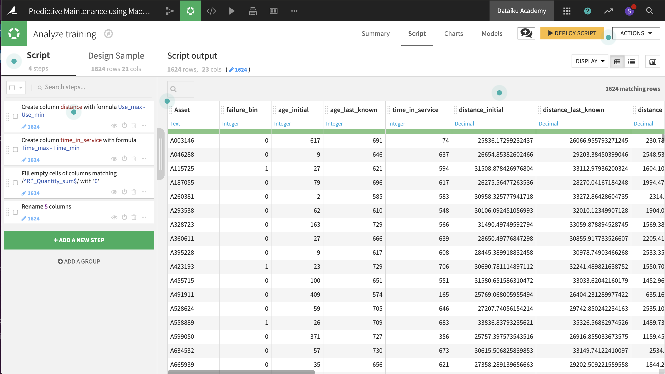
2. Under the Visual Analysis side, select New and accept the default name Analyze training.

3. In the screen which looks similar to a Prepare recipe, create two new variables with the formula processor.

• distance from the expression, Use_max - Use_min

• time_in_service from the expression, Time_max - Time_min

4. Use the Fill empty cells with fixed value processor to replace empty values with 0 in columns starting with Reason. The regular expression ^R.*_Quantity_sum$ is handy here.

5. Lastly, in order to make the model results more interpretable, use the Rename columns processor according to the table below.

Old col name	New col name
count	times_measured
Time_min	age_initial
Time_max	age_last_known
Use_min	distance_initial
Use_max	distance_last_known

Note

It is not necessary to deploy a script created in the Lab to the Flow in order to make use of the new features in the modeling process. Any models created in a Visual Analysis have access to any features created in the same Visual Analysis.

Next, we’ll make some models!

Creating the Prediction Model

Now that we have a dataset ready on which to train models, let’s use machine learning to predict car breakdown.

From the open Lab Script, navigate to the Models tab. If none yet exist, we want to Create our First Model. Dataiku DSS lets us choose between two types of modeling tasks:

1. Prediction (or supervised learning): to predict a target variable (including labels), given a set of input features

2. Clustering (or unsupervised learning): to create groups of observations based on some shared patterns or characteristics

In this case, we are trying to determine whether or not a rental car will have problems. So, opt for a Prediction model.

Dataiku DSS then asks us to select the target variable. In this case, we want to calculate the probabilities for one of two outcomes: failure or non-failure, i.e., perform two-class classification. Accordingly, choose failure_bin as the target variable.

Once we have picked the type of machine learning problem, we can customize the model through either the option of Automated Machine Learning or Expert Mode.

Automated Machine Learning helps with some important decisions like choosing the type of algorithms and parameters of those algorithms. Select Automated Machine Learning and then Quick Prototypes, the default suggestions.

With the default design prepared, clicking Train will build models using the two default algorithms for this type of problem.

Once we have the results of some initial models, we can return to the Design tab to adjust all settings. For example, after navigating to the Basic > Metrics menu in the left sidebar, we can define how we want model selection to occur. By default, the platform optimizes for AUC (Area Under the Curve), i.e., it picks the model with the best AUC, while the threshold (or probability cut-off) is selected to give the best F1 score. Similarly, feature engineering can also be tailored as needed, from which/how features are used, as well as options for dimension reduction.

An important setting is the type of algorithms with which to model the data (under Modeling > Algorithms). In addition, we can define hyperparameters for each of them. For now, we’ll run two machine learning algorithms: Logistic Regression and Random Forest. They come from two classes of algorithms popular for these kinds of problems, linear and tree-based respectively.

Understanding the Model

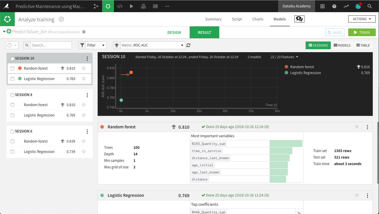
If satisfied with the design of the model, return to the Results tab. Dataiku DSS provides model metrics auto-magically! For example, we can compare how models performed against each other. By default, the AUC is graphed for each model. By that metric, Random Forest has performed better than Logistic Regression.

We can switch from the Sessions view to the Table view to see a side-by-side comparison of model performance across a number of metrics. In this case, Random Forest has performed better across a number of different metrics. Let’s explore this model in greater detail.

From any view in the Results tab, clicking on the name of the model will show us a great deal of under-the-hood insight and ready-made analysis. Besides providing information on features and training and validation strategies, this analysis also helps us interpret the model and to understand its performance.

For example, we can obtain the number of correct and incorrect predictions made by this Random Forest model in a Confusion matrix. We can see the ROC curve used to calculate the AUC, the metric used to select our top model, or explore Detailed metrics.

We can dive into the Decision trees that are aggregated to calculate which features are important and to what extent. At the same time, we don’t want to miss out of the important details of this Random Forest for these trees! So let’s discuss some of the implications of this model.

The Variable importance chart displays the importance of each feature in the model for tree-based methods. Some important ones are, not surprisingly, related to its age and usage. Its time_in_service, as well as its last known age and distance, help predict whether or not the car fails. The last known and total mileage (distance_last_known and distance) are also important. Finally, data from maintenance records are also useful. Among them, R193_Quantity_sum, i.e., the total number of parts used for reason code 193, is important in predicting failure at a later date.

Contextual knowledge becomes critical at this point. For example, knowledge of the rental company’s acquisition strategy for vehicles can discern whether these features are important or why they make sense. For now, let’s use the model to make some predictions.

Using the Model

Let’s use this Random Forest model to generate predictions on the unlabelled scoring dataset. Remember, the goal is to assign the probability of a car’s failure.

1. From within the Lab, select the Model page and find the Deploy button near the top right.

2. Because we created this visual analysis from the training dataset, it should already be selected as the Train dataset in the “Deploy prediction model” window.

3. In the same window, you might change the default Model name to Prediction of failure on training data. Click Create.

4. In the Flow, select the model we just created. Initiate a Score recipe from the right sidebar.

5. Select scoring as the input dataset and Prediction of failure on training data as the Prediction Model. Name the output dataset scored.

6. Create and run the recipe with the default settings.

Note

There are multiple ways to score models in Dataiku DSS. For example, in the Flow, if selecting a model first, you can use a Score recipe (if it’s a prediction model) or an Apply model (if it’s a cluster model) on a dataset of your choice. If selecting a dataset first, you can use a Predict or Cluster recipe with an appropriate model of your choice.

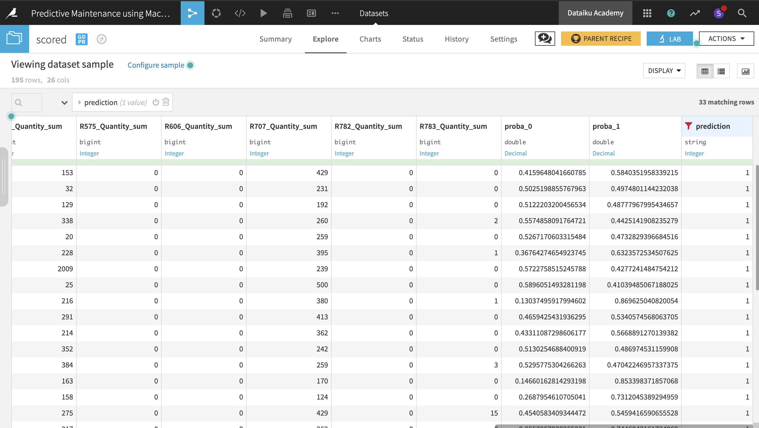
The resulting dataset now contains three new columns:

• proba_1: probability of failure

• proba_0: probability of non-failure (1 - proba_1)

• prediction: model prediction of failure or not (based on probability threshold)

Wrap-up

And that’s a wrap! You can always find the completed project in the Dataiku gallery.

The goal here was to build an end-to-end data product to predict car failures from a workflow entirely in Dataiku DSS. Hopefully, this data product will help the company better identify car failures before they happen!

Once we have a single working model built, we could try to go further to improve the accuracy of this predictive workflow, such as:

• Adding features to the model by combining information in datasets in more ways

• Trying different algorithms and hyper-parameter settings

Also, to make the model more operational, it can be packaged and deployed through a REST API, to be consumed in real time by external applications. It is possible to do so using Dataiku DSS for an end-to-end deployment!