Working with Shapefiles and US Census Data in DSS

This brief tutorial introduces working with shapefiles and US Census data in DSS. It covers importing shapefiles, enriching them with demographic data from the US Census, and mapping the results.

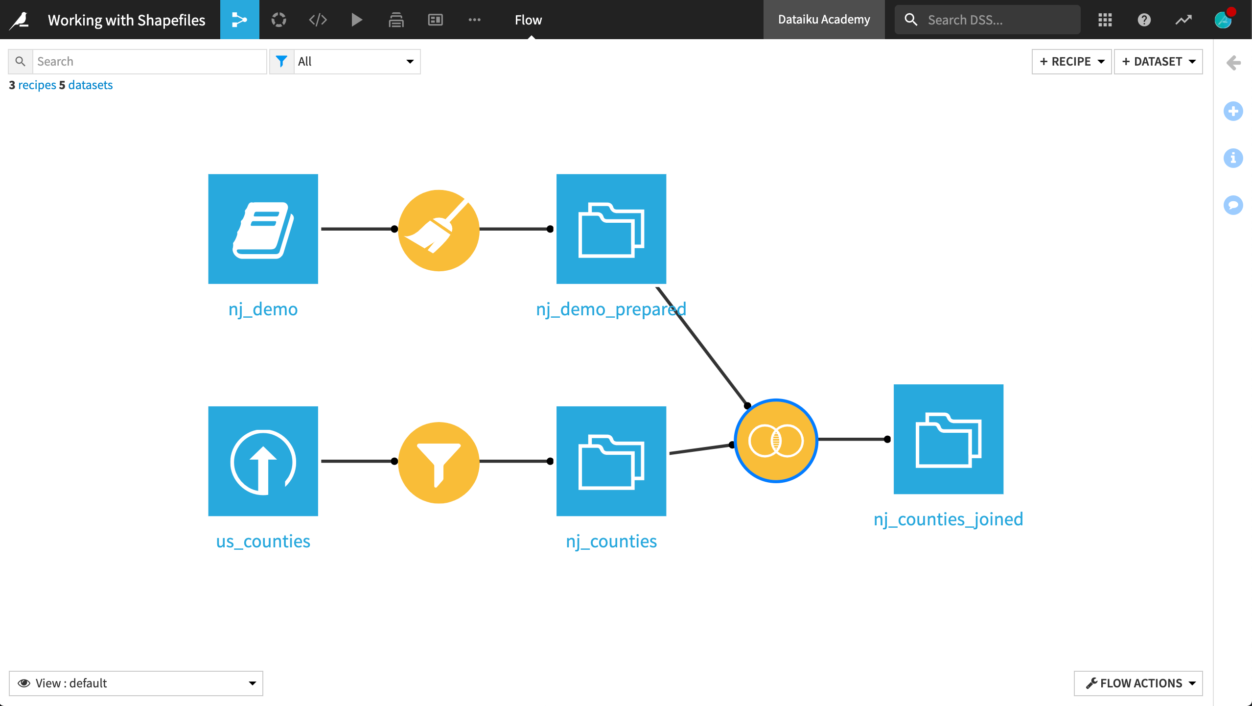
The final project Flow is shown below. A completed version of the project, including the final choropleth, can be found on the Dataiku gallery.

Technical Requirements

• The Reverse Geocoding / Admin maps plugin for producing maps with administrative boundaries

• The Census USA plugin for downloading US Census data

Supporting Data

• The example data for this exercise is TIGER/Line Shapefiles from the US Census Bureau. They contain official 2019 US county borders among some other information, and can be downloaded as a zip archive here.

We will also download US Census data through the Census USA plugin.

The Shapefile Format

When working with spatial or geographic data, you will encounter many different types of file formats such as .geojson, .gpkg, .csv, and .tiff. One of the most common though is the shapefile, initially created by ESRI.

Although often referred to as a singular file, a shapefile is actually a collection of typically four (and potentially other) files (.shp, .shx, .dbf, and .proj).

Together, these files can spatially describe vector features such as points, lines and polygons.

Importing Shapefiles

Dataiku DSS provides built-in support for the shapefile format.

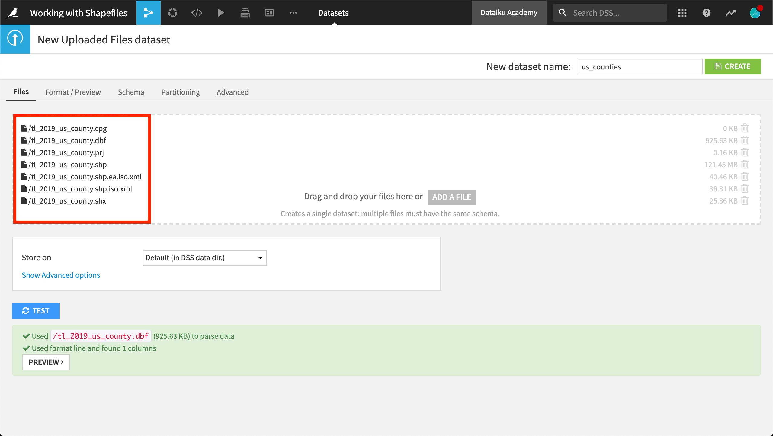
In a new blank project, (we’ve named ours Working with Shapefiles), create a new dataset by uploading the downloaded zip archive to DSS.

• On the Format/Preview tab, ensure the selected Type is Shapefile, if not already done so.

• Create the new dataset with the name us_counties.

Exploring Shapefiles

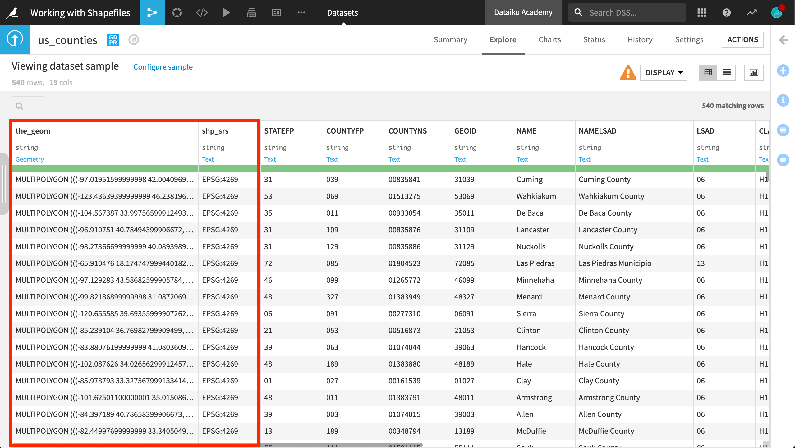
After importing the dataset, the Explore tab shows a preview of the data in a tabular format.

The first column, the_geom, specifies the dataset’s geometry.

• It is stored as a string, but DSS can interpret its meaning to be Geometry. Each row, a county, is stored as a multipolygon.

The second column, shp_srs, specifies the dataset’s Spatial Reference System (SRS), also known as a Coordinate Reference System (CRS).

• A spatial reference system defines how the spatial elements of the data relate to the Earth’s surface. In this case, the dataset uses one of the most common geographic SRS, EPSG:4269.

Shapefiles in a Visual Recipe

Shapefiles can be manipulated in DSS like any other dataset. Let’s use it in a visual recipe.

• From the us_counties dataset, initiate a Sample/Filter recipe.

• Name the output dataset nj_counties.

• Filter the dataset to keep only rows where STATEFP equals 34, the FIPS code for the state of New Jersey.

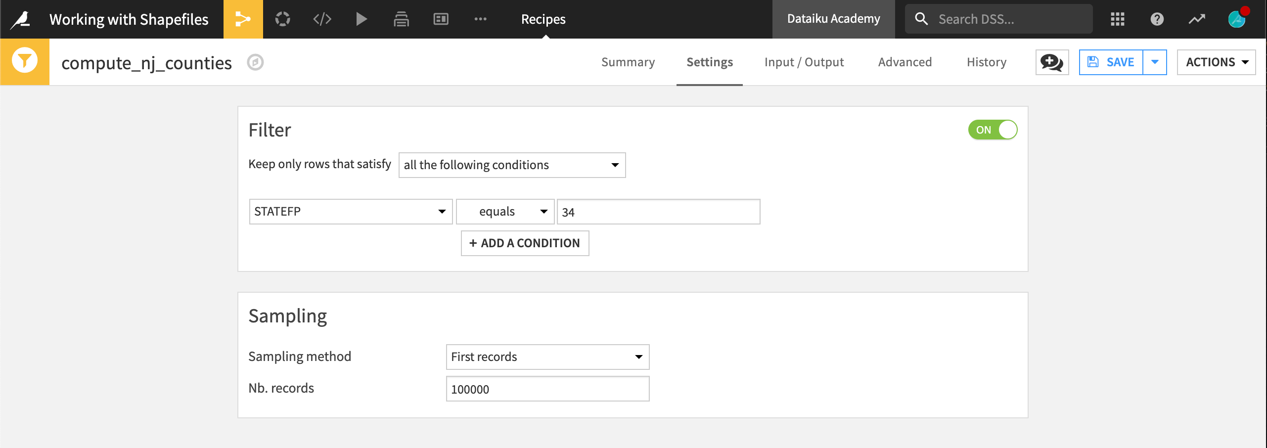
After running the recipe, note that the output dataset now has 21 rows, one for each county in New Jersey.

Note

Note that the same result of the Filter recipe could be achieved with a Filter rows/cells on value processor in a Prepare recipe.

Downloading US Census Data

We now have a dataset where each row holds the shape of a county in New Jersey. As of now though, there is no demographic data attached to the counties.

The Census USA plugin has a number of features relating to Census data, including an easy way to download data from the US Census Bureau.

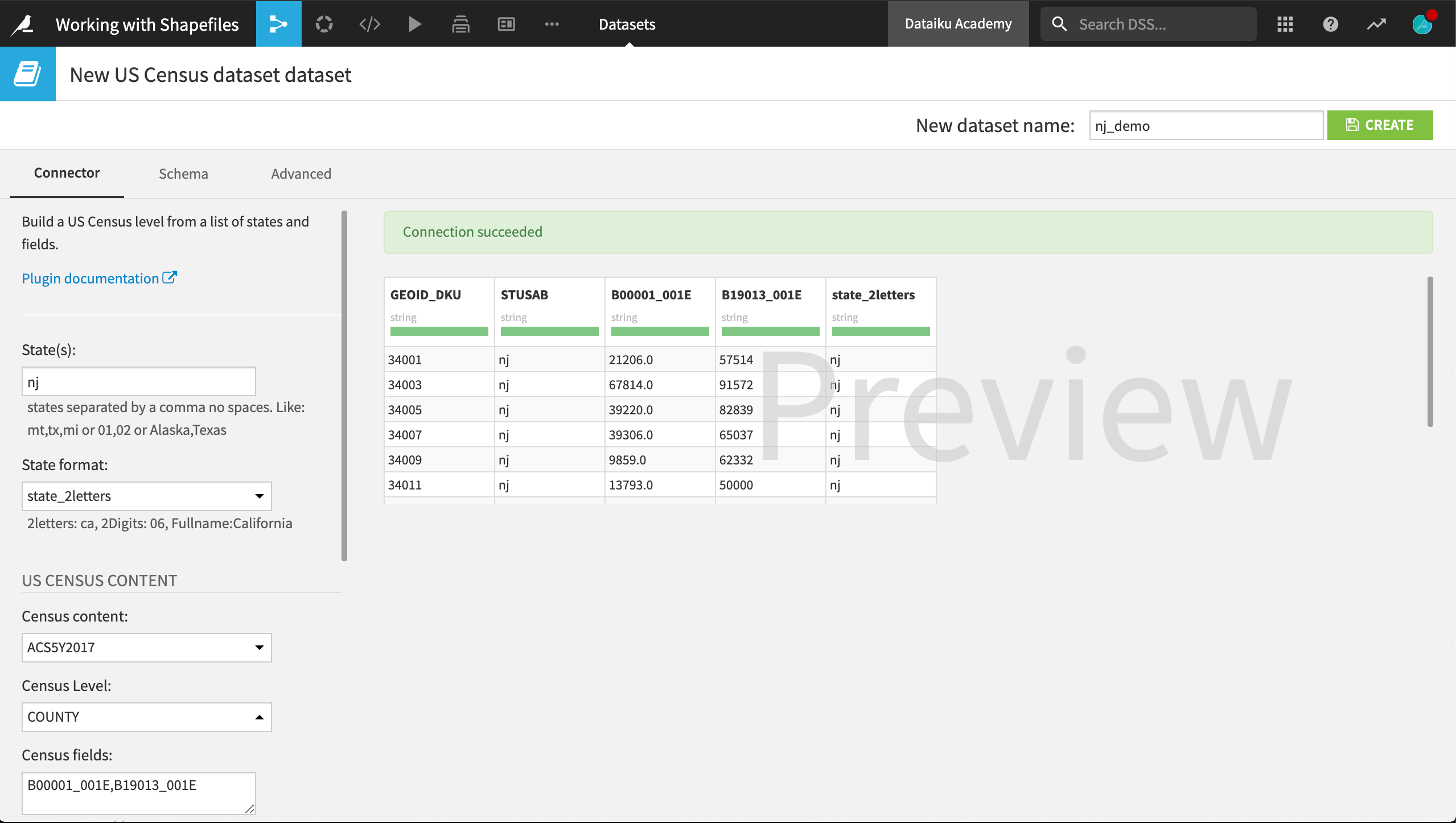
• From the Flow, select + New Dataset > Census USA > US Census dataset.

• For the “State”, provide nj. Ensure “State format” is state_2letters.

• Select ACS5YR2017 as “Census content” and County as “Census level”.

• The “Census field” is a string of variables (without spaces). Add B00001_001E,B19013_001E to retrieve data for total population and median household income, respectively.

• Click “Test & Get Schema”.

• Name the output dataset nj_demo.

Once this dataset has been created, we now have the population and an estimate of median household income for each county in the state.

Note

There are a number of ways to find out the code for a particular census variable. One way is by building the US Census metadata dataset in the Census USA plugin.

Enriching Shapefiles with Census Data

Before we can join our spatial and demographic data, we’ll do a few brief preparation steps on the demographic data.

• Initiate a Prepare recipe on nj_demo.

• Rename the variable code columns so they are easier to remember.

  • Rename B00001_001E to population.

  • Rename B19013_001E to med_household_income.

• We also want to edit the Schema in the Settings tab so that GEOID_DKU is a string. Although this column may look numeric, we cannot do any calculations with these “numbers”. Moreover, the GEOID column of nj_counties is stored as a string, and we’ll use these two columns as the join key.

We can now join the datasets of shapefiles and demographic information as we would any two datasets.

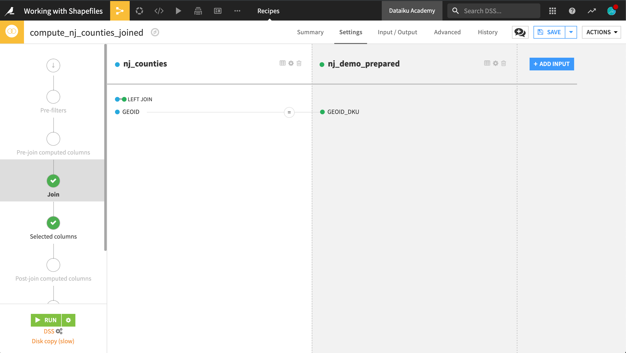
• In a Join recipe, left join nj_demo_prepared to nj_counties.

• In the Join step, use the GEO_ID column of nj_counties and the GEOID_DKU column of nj_demo_prepared as the key.

• In the Selected columns step, retain only population and med_household_income from nj_demo_prepared.

Running the recipe should produce an output dataset with two additional columns, the population and the median household income for each county.

In this case, you can ignore the INPUT_DATA_VERY_LONG warning. We can see that DSS is just warning that the column holding the geometry of our shapefile is unusually large (compared to a typical column).

Mapping Shapefiles

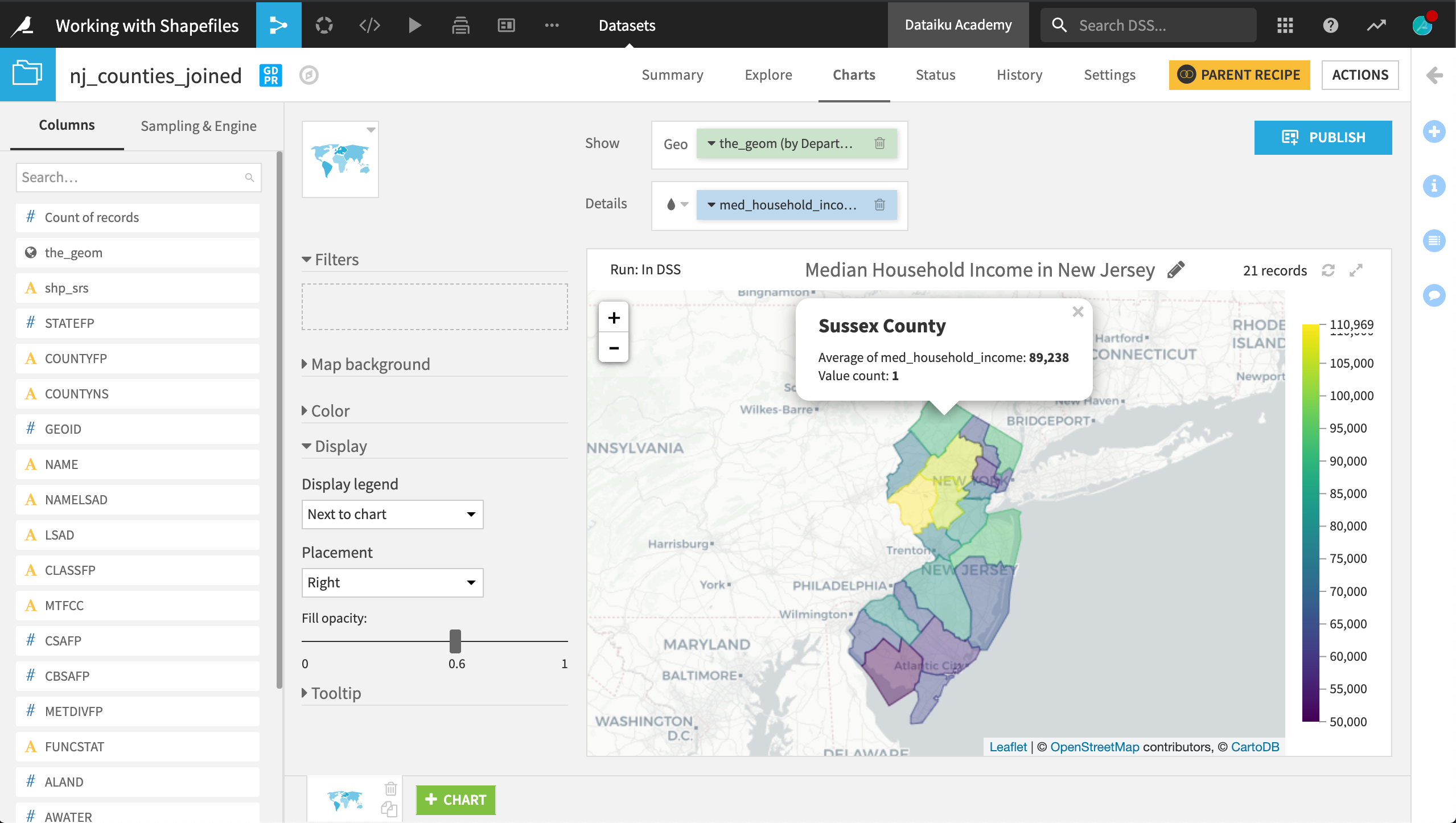
Now we can visualize the distribution of our demographic variables on a map.

• On the Charts tab of the nj_counties_joined dataset, create a Filled Administrative map.

• Drag the_geom column to the Geo field. Adjust the level of detail from Country to Department/County.

• Drag the population or med_household_income column to the color droplet field.

• Adjust the color palette to your preference.

What’s Next?

Congratulations! You’ve seen how to import, manipulate, and visualize shapefiles and US Census data in DSS.

Recall that you can find the completed version of this project in the Dataiku gallery.

Next, you might be interested in turning this map into a web app that can allow end users to toggle between variables.