Concept Summary: Classification Algorithms

In this lesson, we’ll learn about a type of supervised learning called classification. Specifically, we’ll look at some of the most common classification algorithms: logistic regression, decision trees, and random forest.

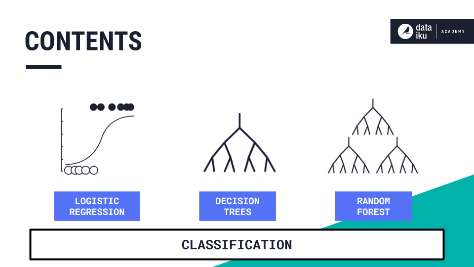
Classification refers to the process of categorizing data into a given number of classes. The primary goal is to identify the category or class to which a new data point will fall under.

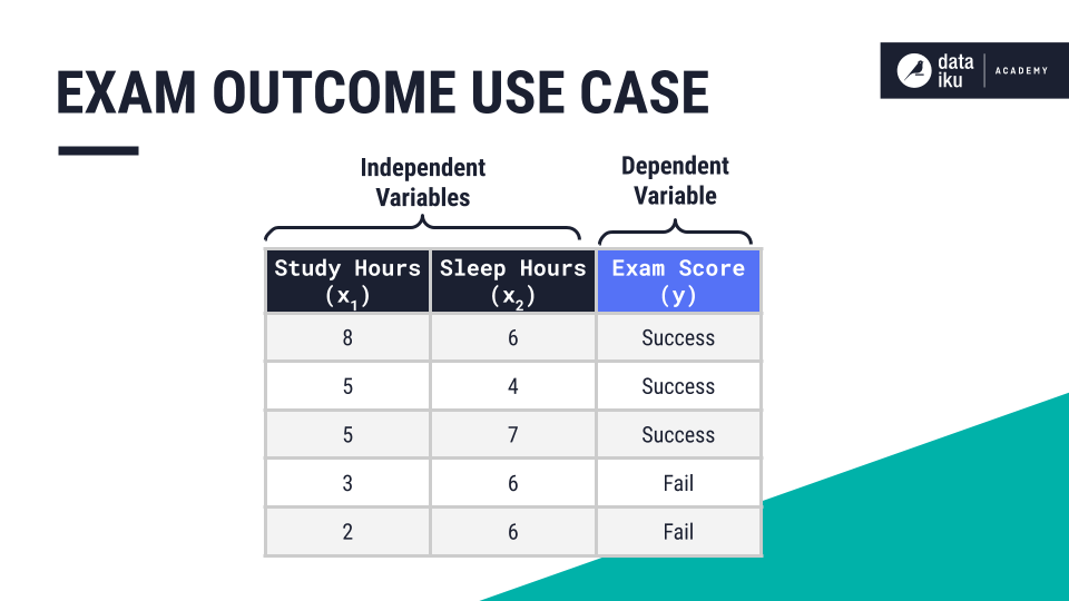
In our use case, the target, or dependent variable, is the exam outcome. The features, or independent variables, are study hours and sleep hours. The target is what we are trying to predict.

Logistic Regression

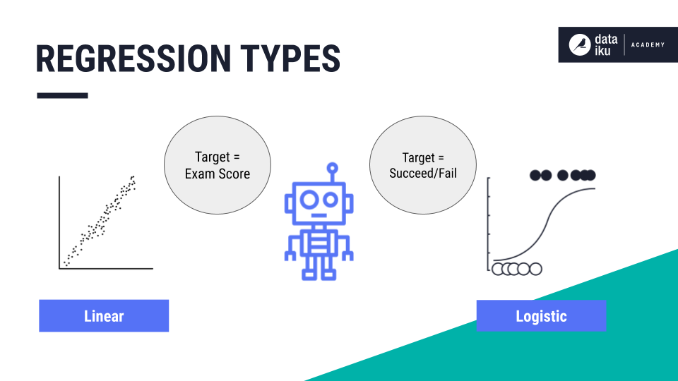
Let’s compare logistic regression with linear regression. Linear regression is a prediction algorithm we learned about in the Regression section. In linear regression, we attempt to predict the student’s exact exam score. This generates a straight line of best fit to model the data points.

With logistic regression, we attempt to predict a class label–whether the student will succeed or fail on their exam. Here, the line of best fit is an S-shaped curve, also known as a Sigmoid curve.

In logistic regression, we use this S-shaped curve to predict the likelihood, or probability, of a data point belonging to the “succeed” category. All data points will ultimately be predicted as either “succeed” or “fail”.

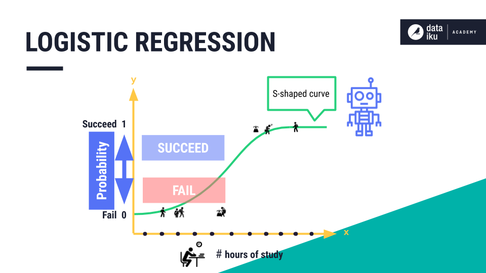
In order to generate the final class prediction, we need to use a pre-defined probability threshold. All data points above the probability threshold will be predicted as “succeed”, and all data points below will be predicted as “fail”. For example, our model tells us that at five hours of study, there should be about a 45% probability of a student succeeding on their exam.

But depending on where we set the threshold, this student’s outcome could be classified as either “succeed” or “fail”.

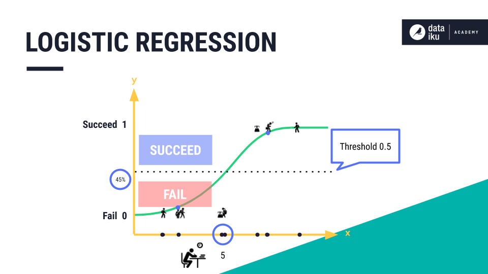
For example, if the threshold was set at the halfway mark, or 0.5, the student would be classified as “fail”. If we changed the threshold, to say 0.4, then the student would be classified as “succeed”.

We could use a confusion matrix to help us determine the optimal threshold. As we discovered in the lesson, Model Evaluation, a confusion matrix is a table layout used to evaluate any classification model.

Decision Trees

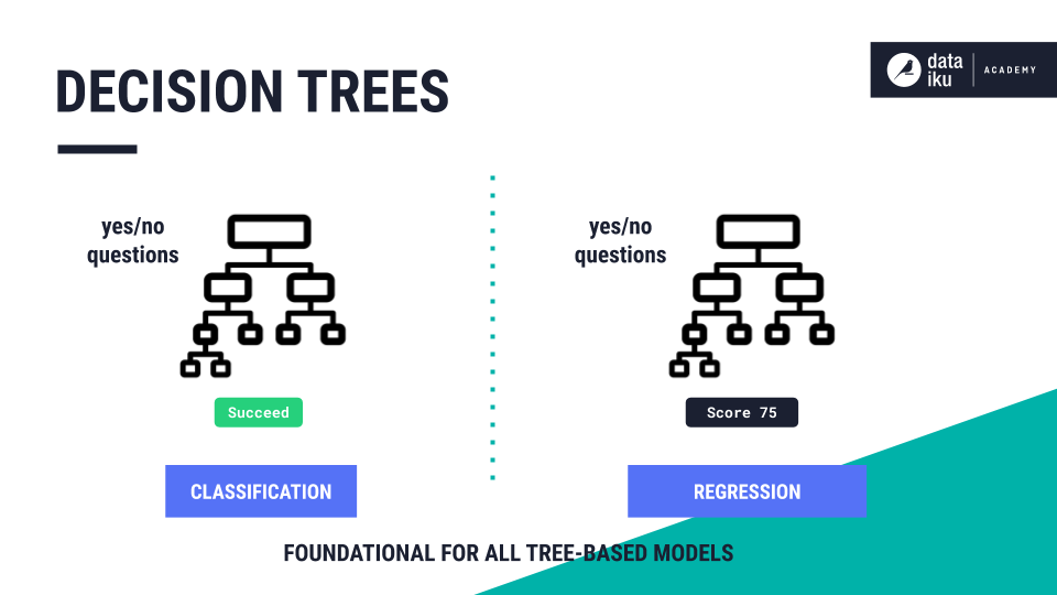
Decision Trees are another type of algorithm most frequently used for classification. Decision trees can also be used for regression. Instead of being limited to a single linear boundary, as in logistic regression, decision trees partition the data based on either/or questions.

When decision trees are used In classification, the final nodes are classes, such as “succeed” or “fail”. In regression, the final nodes are numerical predictions, rather than class labels. A decision tree is the foundation for all tree-based models, including Random Forest.

Building a Decision Tree

Using our Student Exam Outcome use case, let’s see how a decision tree works. We’ll add a few more input variables, or features, to the student data set we used for our logistic regression problem. The new features are “healthy diet” and “study group”.

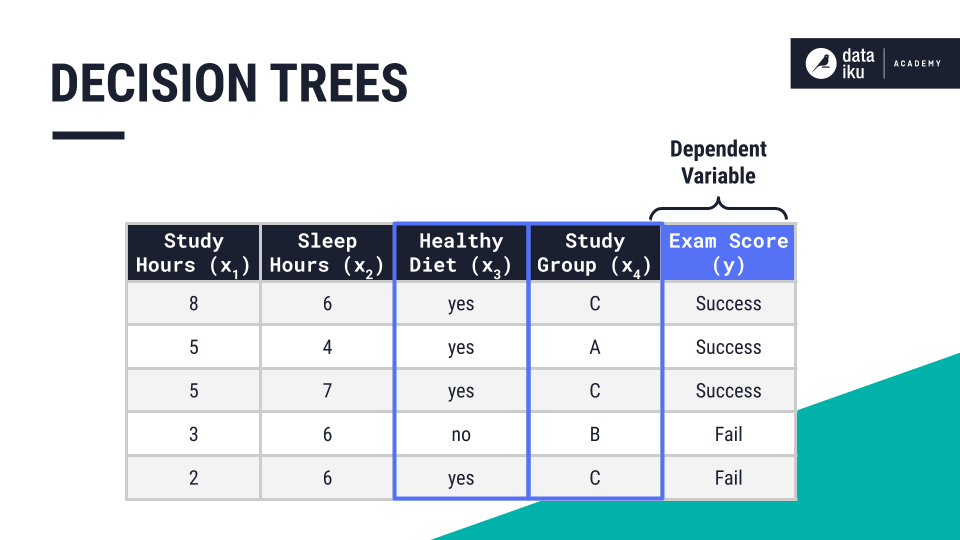
A decision tree is an upside-down tree where the root and the branches are made up of decisions, or yes/no questions. In our Student Exam Use Case, our tree creates each split by maximizing the homogeneity, or purity, of the output datasets. For example, our tree might start by splitting the dataset into two—based on a yes/no question (also known as a feature): “Did the student study less than 5 hours?”.

This is a good place to split. When comparing the group of students who studied more than five hours to the group who studied less than five hours, the two datasets are relatively pure and have low variance.

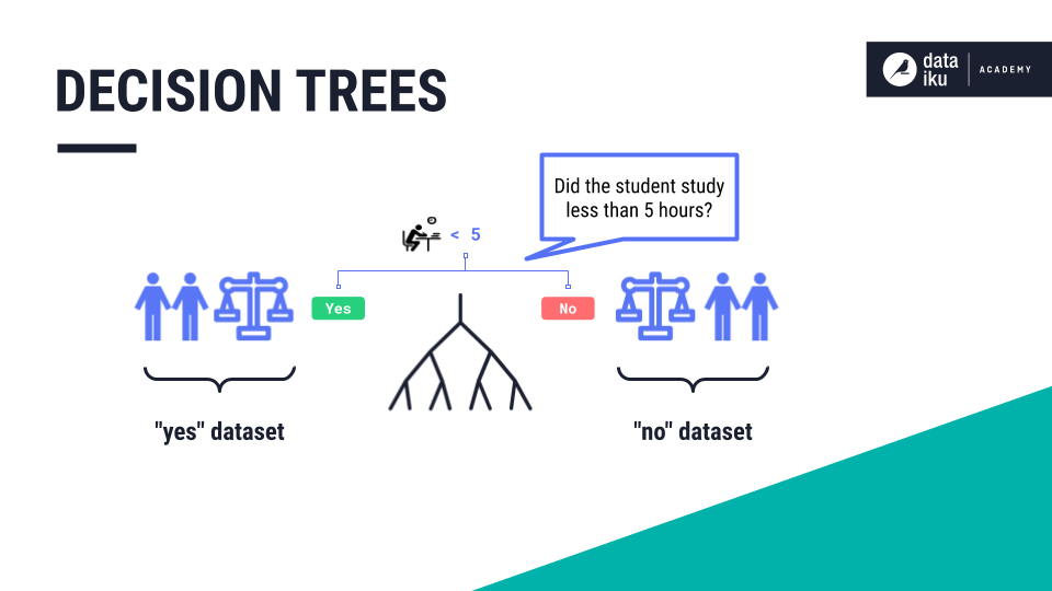
Starting with study hours as the root of the tree, let’s follow one student data point through each yes/no question, or decision node, in the tree. Our first question is whether the “hours of study” were “less than or equal to 5”. This student studied for eight hours and so the answer is “no”.

From this answer, we create a branch where we move on to the next node, or question: “Did the student sleep less than 5 hours?”.

Based on the answer, “no”, we can create another branch for our next node, or question: “Did this student eat a healthy diet?”.

Here, the answer is “yes”. We create another branch and move on to the next question: “Was this student a part of Study Group C?”.

This student was a part of study group C. We create another branch and move on to the next node, or question, and so forth.

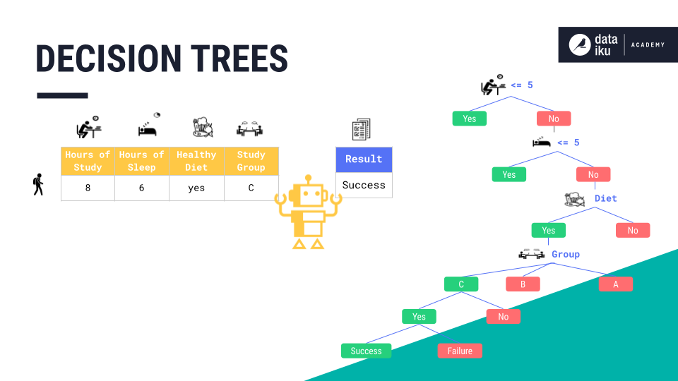
The machine has learned a new rule: “Students who study more than five hours, sleep more than five hours, eat a healthy diet, and are part of group C are likely going to succeed on the exam.” In this use case, the tree ended at a final prediction–or class label–“success.”

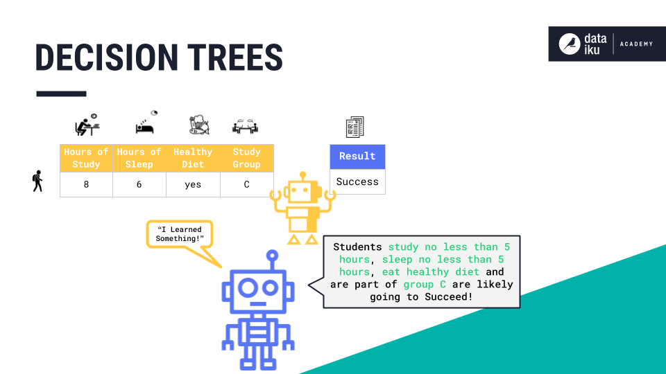
After the model has been trained on all records of the training set, the machine learning practitioner can validate and evaluate it. If the results are satisfactory, then the practitioner can apply the model to new, unseen data.

Pruning

A technique called “pruning” can help improve our model and avoid overfitting. Pruning refers to the process of removing branches that are not very helpful in generating predictions.

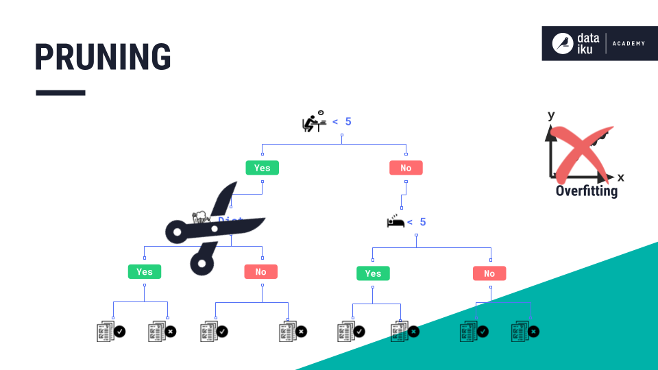
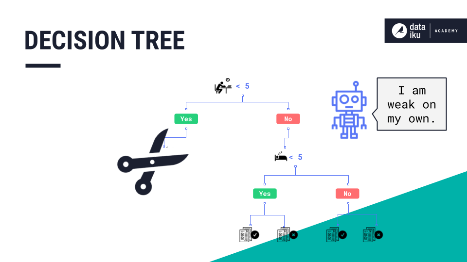
Pruning is a good method of improving the predictive performance of a decision tree. However, a single decision tree alone will not generally produce strong predictions by itself.

Random Forest

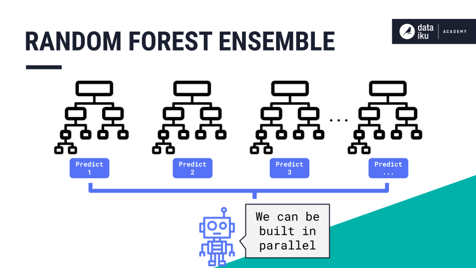
A random forest is an ensemble of decision trees where many trees, which may be weak on their own, come together to generate one strong guess. Each tree represents randomness: (a) because the dataset sample used to build it is random, and, (b) the subset of the model’s features used to evaluate each split is random. The trees are not correlated with one another in any way, and they can be built in parallel.

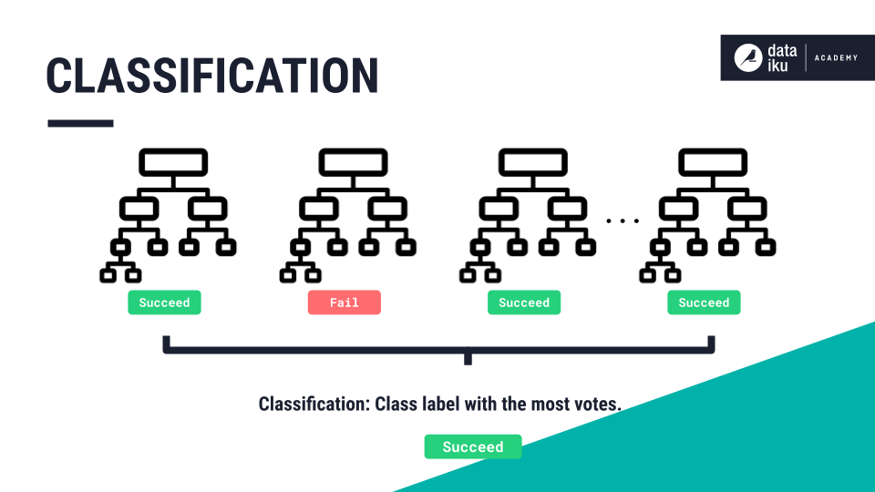
In classification problems, the class label with the most votes is our final prediction.

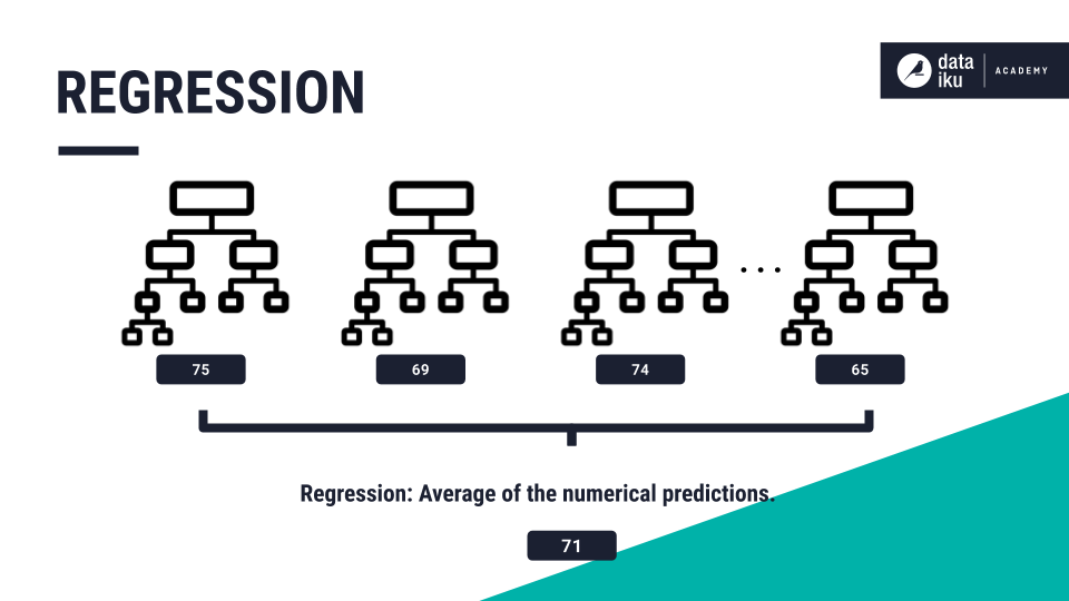
In regression problems the final prediction is an average of the numerical predictions from each tree.

Summary

In this lesson, we discussed common classification algorithms including logistic regression, decision trees, and random forest.

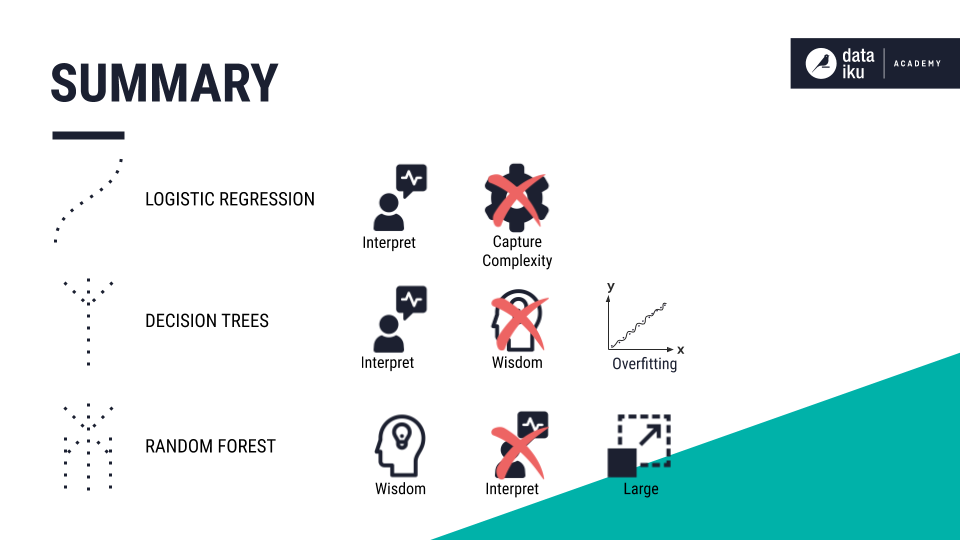
Logistic regression is easy to interpret but can be too simple to capture complex relationships between features. A decision tree is easy to interpret but predictions tend to be weak, because singular decision trees are prone to overfitting. Finally, random forest is a sort of “wisdom of the crowd”. However, it is not easy to interpret and models can get very large.

What’s next

Now that you’ve completed this lesson about classification algorithms, you can move on to discussions about an unsupervised learning technique–clustering.