Visual Window Analytic Functions

Although it may be possible to code window functions in languages like R and Python, they typically run more efficiently in SQL (and SQL-like: Hive, Impala, Spark, etc.) databases. They are also one of the least known and trickiest to code successfully.

The Window visual recipe in Dataiku allows you to take advantage of these powerful features without coding. For example:

• Filtering rows by order of appearance within a group

• Computing moving averages, cumulative sums, and rankings

• Computing the number of events that occurred during the n days prior to another event

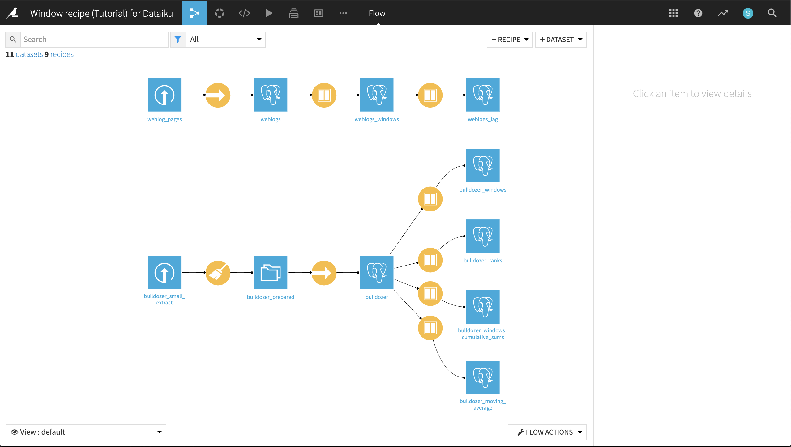
This tutorial demonstrates how to implement many of these calculations using the Window recipe. The final project after completing the tutorial can be found in the Dataiku gallery. The final project Flow appears below.

Conceptual Understanding

The PostgreSQL documentation has a very good introduction to the concept of Window analytics. Quoting:

Note

Definition of a window function

A window function performs a calculation across a set of table rows that are somehow related to the current row. This is comparable to the type of calculation that can be done with an aggregate function. But unlike regular aggregate functions, use of a window function does not cause rows to become grouped into a single output row — the rows retain their separate identities. Behind the scenes, the window function is able to access more than just the current row of the query result.

In other words, unlike a Group recipe, a Window recipe does not reduce the number of rows in a dataset. It creates new columns in a dataset that are the results of computations that use all rows in a “window”, that is, a subset, of all rows of the dataset.

Conceptually, there are two steps when defining a window recipe:

• Defining the window(s): On what rows of the dataset will the computations apply?

• Defining the aggregation(s): What do I compute on this window?

The window can be:

• Partitioned: Define one or several columns, and one window is created for each combination of values of these columns.

• Bounded: For each row, restrict the window to start:

  • at the beginning (resp. to the end)

  • at a given number of rows before the current row

  • at a given range of values before a given column of the current row

  • at the current row

The same bounding can be applied to the end of the window. In addition, a window can be ordered (this is actually required for bounding it).

Create Your Project

From the Dataiku home page, click +New Project > DSS Tutorials > Visual recipes > Window recipe (Tutorial).

There are two datasets:

• an extract from the “Blue book for Bulldozers” Kaggle competition data.

  • Each row represents the sale of a used bulldozer. We’re interested in the saledate column from this dataset, but it is an unparsed text string.

  • Start a Prepare recipe and create a new output dataset called bulldozer_prepared. Parse the saledate column, and run the recipe.

• an extract of a web log, containing events where users switch from one page to another

Warning

In order to complete this tutorial, please sync the provided datasets to a database or distributed system using the Sync recipe. Do not store data into your local Filesystem. For details on syncing a dataset to a database, please review the SQL in Dataiku tutorial, which includes a walkthrough of connecting to PostgreSQL in Dataiku.

While syncing the datasets to a PostgreSQL database, we have renamed them to bulldozer and weblogs, respectively.

Adding Average Price as a Column

The bulldozer dataset contains one row per sale, with information about the sale date, price and other particulars of a given bulldozer. For this first example, we want to explore the average price of all bulldozers in the same ProductGroup category.

However, instead of reducing the dataset to the average price of each ProductGroup with a Group recipe, we can use a Window recipe to insert the sale average of a given ProductGroup into the dataset.

Accordingly, with the bulldozer dataset selected, choose Actions > Window and create a new Window recipe.

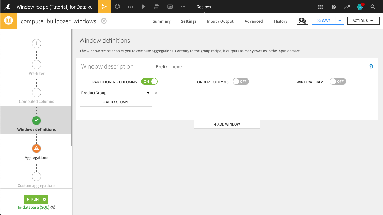
The recipe opens on the Windows definitions step. Here, we are interested in exploring prices relative to ProductGroup so that is the partitioning column. For now, leave the Order Columns and Window Frame settings turned off.

• Activate Partitioning Columns

• Select the ProductGroup column

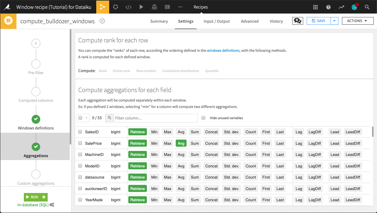
Let’s now move on to the Aggregations step.

We want to Retrieve all columns of the dataset (keep all existing data), and add one new column: the average value of SalePrice. Check the SalePrice > Avg box.

Click Run and accept the schema change warning. The output dataset should include a new SalePrice_avg column.

Using the Analyze tool on the ProductGroup column helps us verify that we have six distinct values, one for each ProductGroup.

With this new column, we could now compute, for example, the difference between the average price of the ProductGroup and the SalePrice of an actual bulldozer, to get a notion of whether any particular bulldozer may be “overpriced”.

Computing Ranks

Continuing with this “overpriced” notion, let’s assign a rank to bulldozers in terms of the most expensive SalePrice within a respective ProductGroup.

Reopen the Window recipe and navigate to the Aggregations step. Note how we are unable to compute ranks for rows. This is because, in the previous Windows definition step, we chose not to order columns. Let’s do this now.

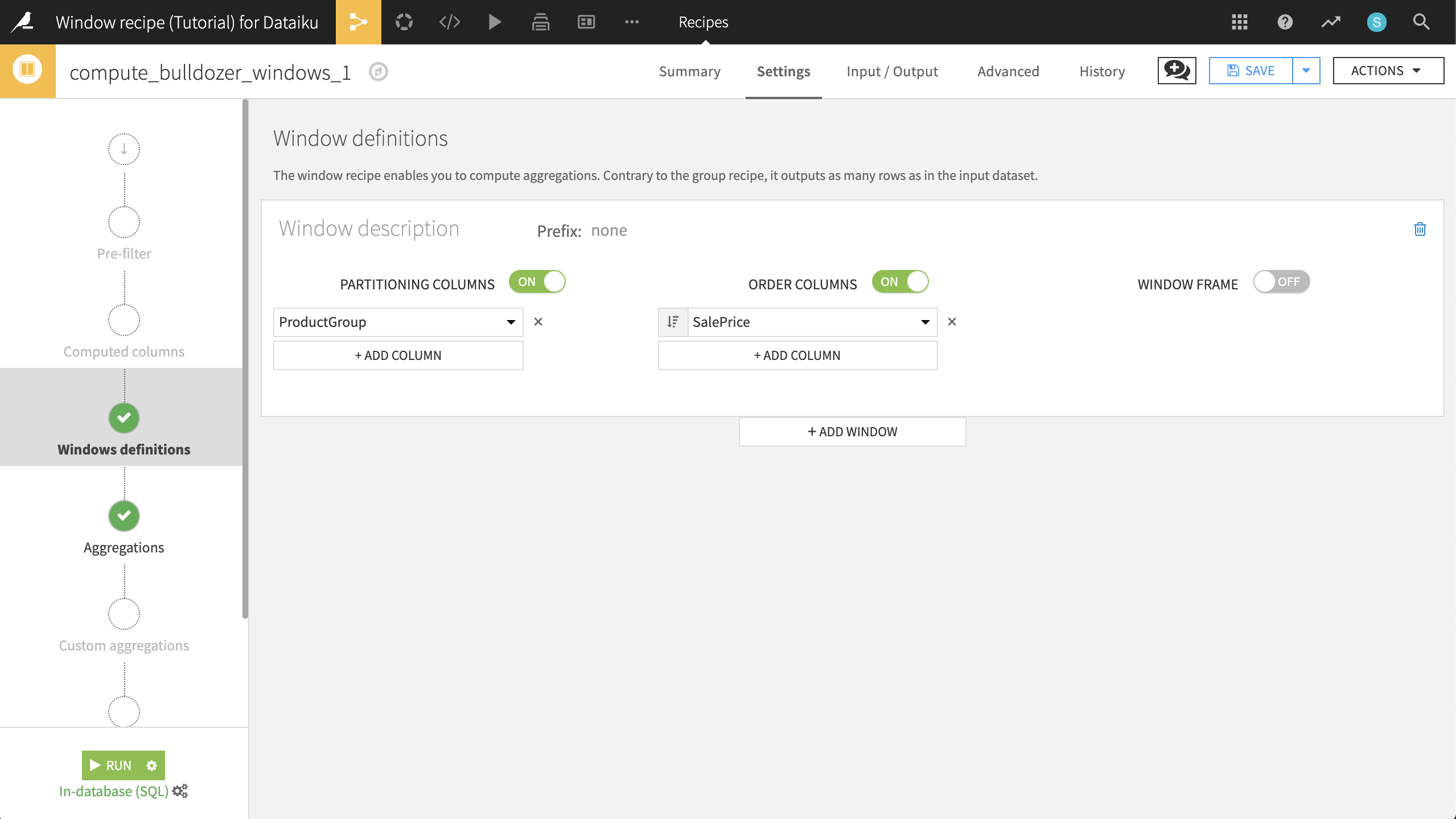
Copy the compute_bulldozer_windows recipe, and name the output dataset bulldozer_ranks. In the Windows definitions step, turn on Order Columns. Select SalePrice as the column to order by, and click the ordering icon so that values are sorted in decreasing order.

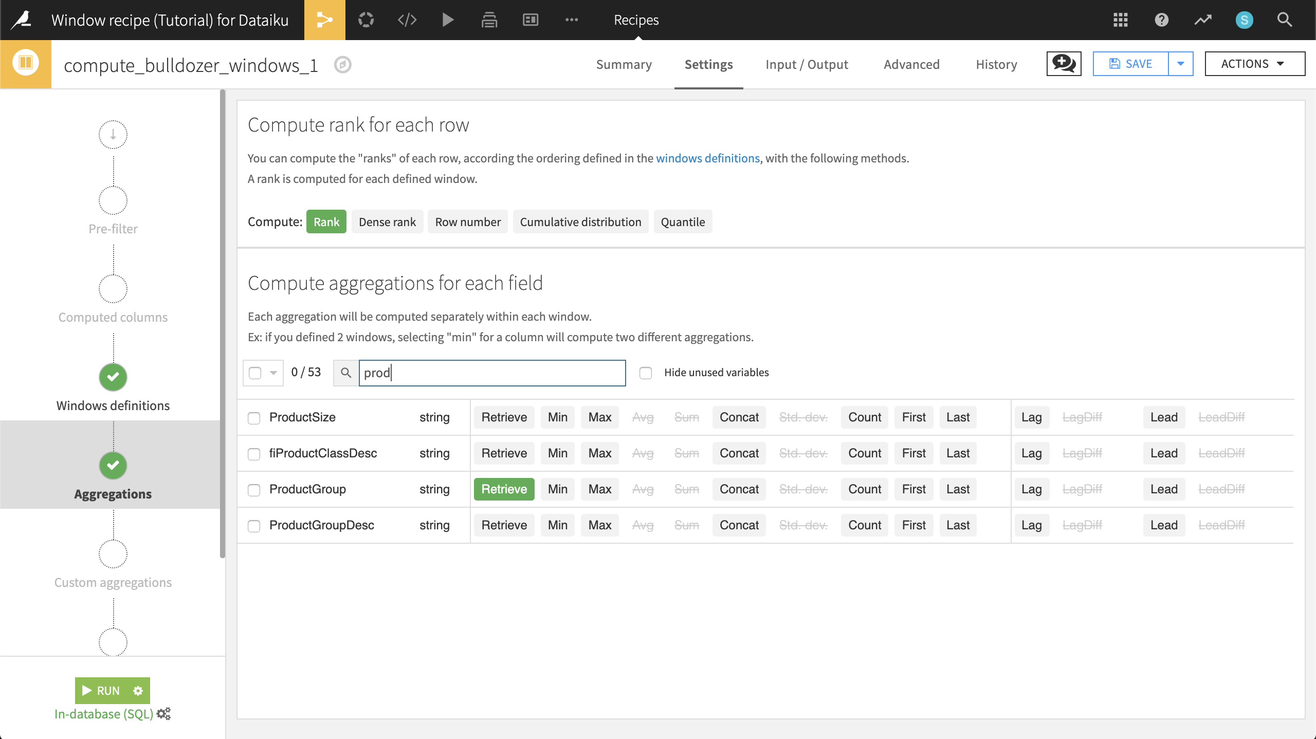
Now go to the Aggregations step. We’ve decided that we want to focus on SalesID, SalePrice, and ProductGroup. We can quickly disable Retrieve original value for all columns, and then add it back for the three we’re interested in. The Avg of SalePrice should also remain.

In addition to computing aggregations based on the fields in the window, we have a few options to compute different types of ranks for each row.

Rank is the “index” of the current row within its window. In other words, since we have a window, partitioned by ProductGroup, and ordered by decreasing SalePrice, the most expensive bulldozer of each ProductGroup will have rank=1, the second most expensive of each group will have rank=2, and so on.

Enable Rank and run the recipe, accepting the schema change.

The resulting dataset is sorted by ProductGroup and descending SalePrice, and the most expensive “BL” bulldozer has a rank of 1. Because we have ordered columns by SalePrice, the SalePrice_avg column is a running average reflecting the sale price average of all rows up to and including the present row.

At this point, we notice two important things:

• First of all, the ranks are not continuous. That’s because we need to break the ties. There are three variants of rank:

  • Rank will output 1,1,3,3,3,6

  • Dense rank will output 1,1,2,2,2,3

  • Row number will output 1,2,3,4,5,6 (ties are broken randomly)

• It may seem strange that the SalePrice_avg now changes within a group. This is because we have ordered columns by SalePrice. The definition of the window automatically changes, becoming bounded between the “beginning” and “current row”. In other words, the average price is computed for each bulldozer by only using the data of the more expensive ones (since the window is ordered by decreasing price). Like SalePrice, we can see that SalePrice_avg is also decreasing.

Cumulative Sums

We’d now like to know the proportion of the total sales made as time passes. In other words, we want to compute the cumulative distribution of the summed price. We’re no longer interested in ProductGroup; we want global information.

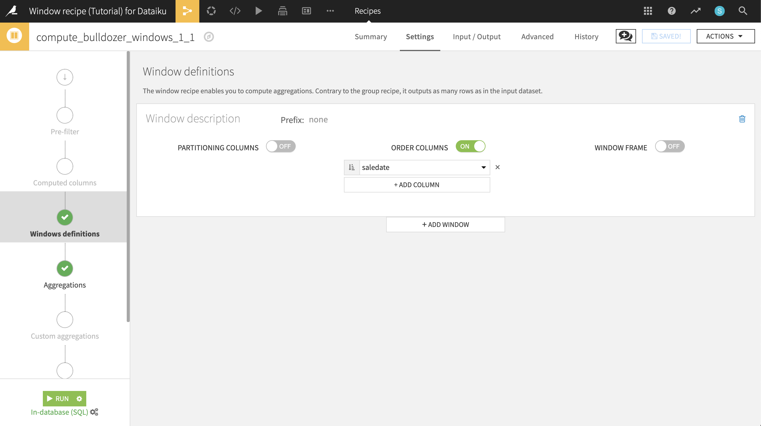
Return to the previous Window recipe used to compute bulldozer_ranks and make a copy. Name the output dataset bulldozer_windows_cumulative_sums, and click Create recipe.

In the Windows definitions step, turn Partitioning Columns off. Change the Order Column to saledate, and click the icon so that dates are sorted in increasing order.

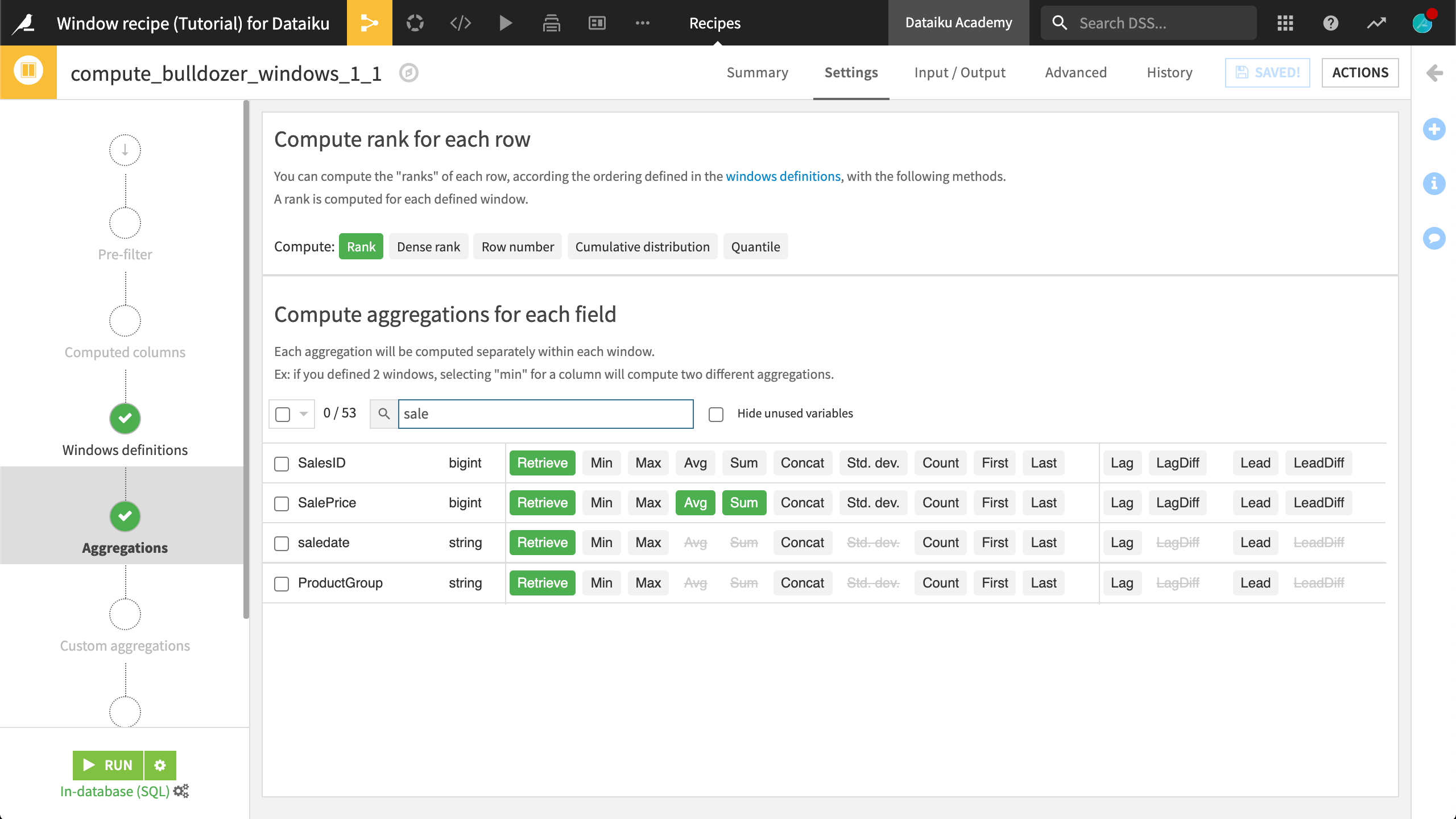
In the Aggregations step, check the SalePrice > Sum box. Since the window is ordered, for each bulldozer, this will compute the sum of the sale price of all previous bulldozers, plus this one.

To better see what’s going on, also check saledate > Retrieve, giving 7 output columns.

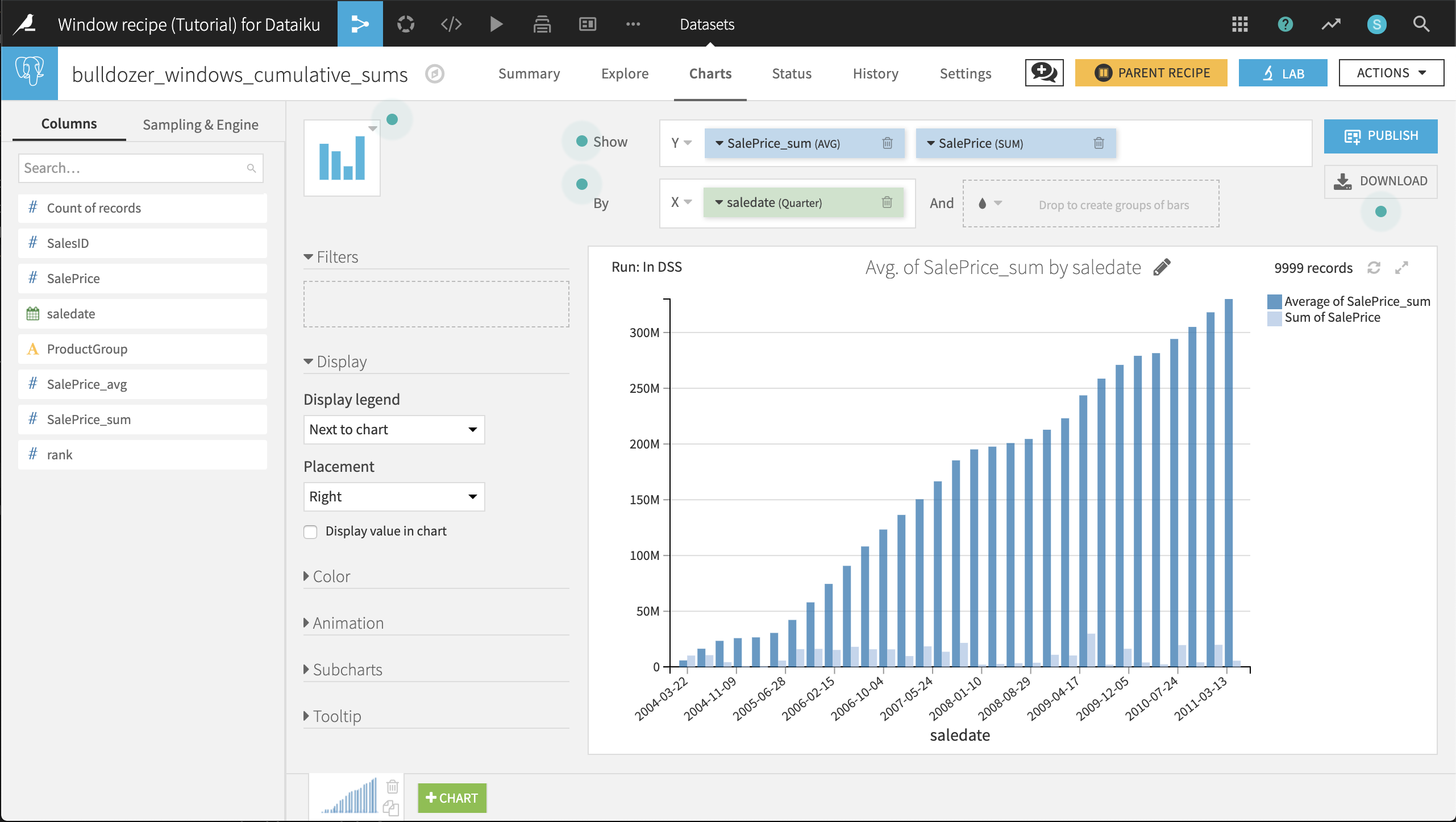
Run the recipe. In the resulting dataset, on the Charts tab, we can chart the cumulative sums along with the marginal increases in the cumulative sum.

• Select SalePrice_sum and SalePrice as Y-axis columns. Set the aggregation to SUM for SalePrice and to AVG for SalePrice_sum.

• Select saledate as the X-axis column. Set the date range as Quarter.

Moving Averages

Thus far, we have seen in action the Partitioning Columns and Order Columns features of the Window recipe. Now let’s utilize the Window Frame feature.

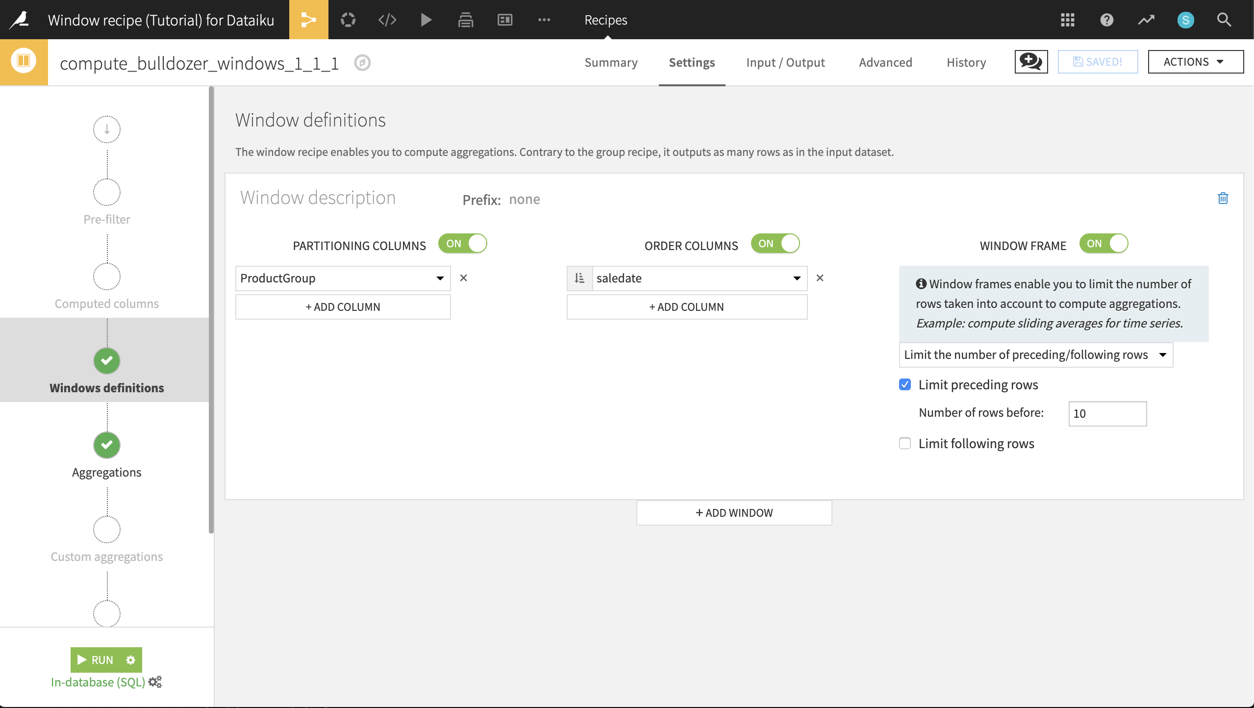
In order to gain a glimpse of how the market is moving, let’s create a moving average of the 10 previous sales for a bulldozer in the same ProductGroup. To do this, we’ll use the Window Frame feature to limit the window to the 10 rows preceding the current row (up to the current row).

Return to the previous Window recipe used to compute bulldozer_windows_cumulative_sums. Make a copy of the recipe, and name the new output dataset bulldozer_moving_average.

In the Windows definition step of the new recipe:

• Turn Partitioning Columns back on, and ensure the ProductGroup column is selected.

• Turn Window Frame on, and limit the preceding rows to 10.

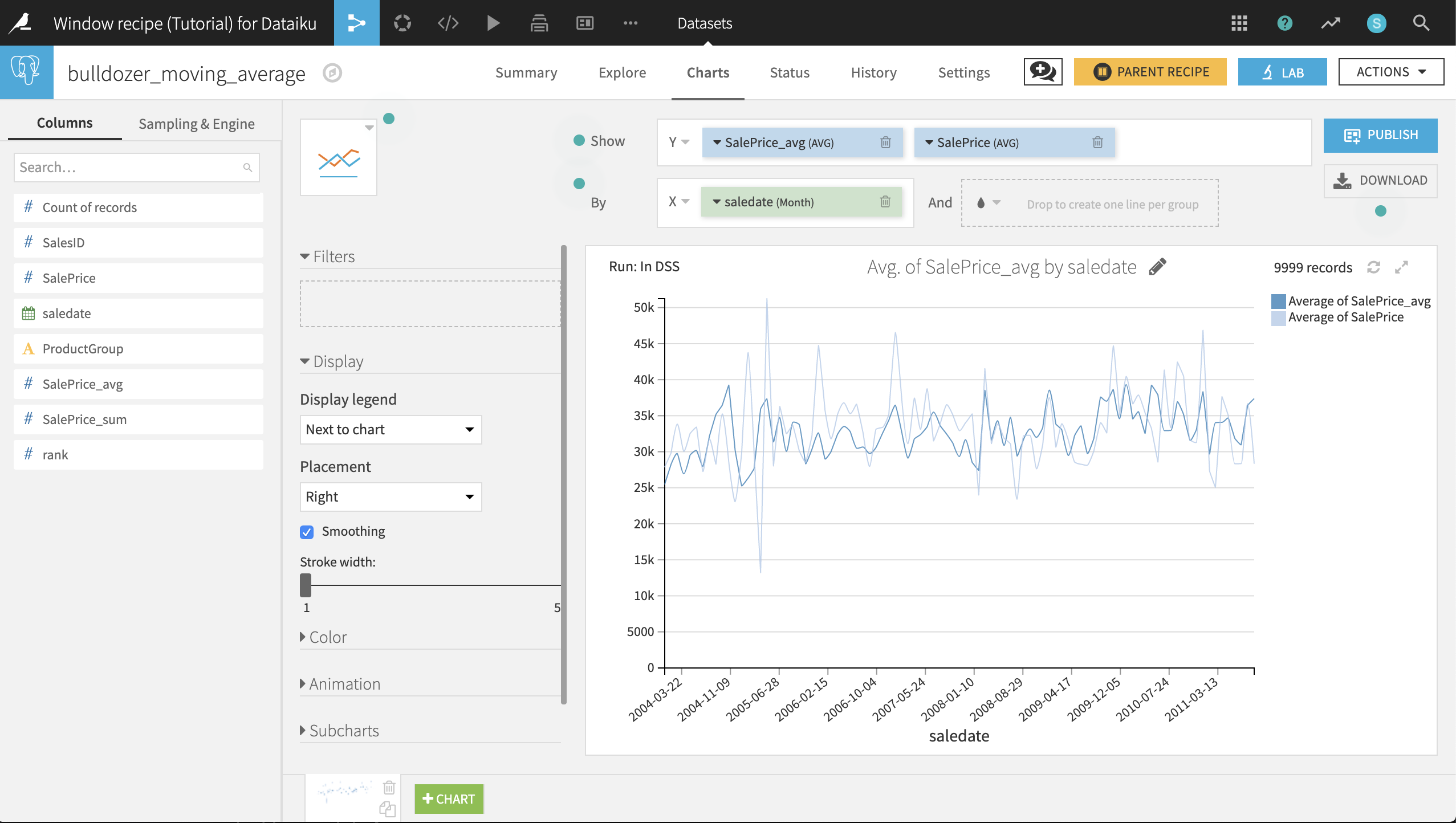
Run the recipe. In the resulting dataset, on the Charts tab, we can chart the moving average along with the monthly average.

• Choose Lines as the chart type.

• Select SalePrice_avg and SalePrice as Y-axis columns. Ensure the aggregation is set to AVG.

• Select saledate as the X-axis column. Set the date range as Month.

Filtering Sessions with Rank

Let’s switch to the weblogs dataset. It contains events on a website. For each event, we have:

• server_ts: the timestamp

• visitor_id: the unique identifier of the visitor

• session_id: automatically resets each time a visitor returns to the site

• page_id: the name of the page on the site

• sc_width: the screen width

• sc_height: the screen height

In web log data such as this, there can be several events on the same page. For example, a user clicking a button on a page might trigger an event. Imagine we want to keep only the first event on each page for each session, regardless of whether the user went back to the page. Window functions can do that!

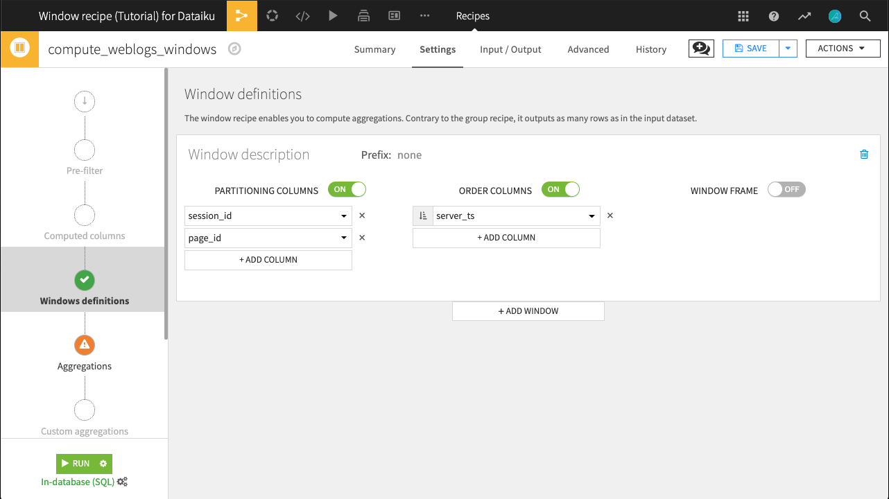
Create a Window recipe (the default output name of weblogs_windows is fine) with the following settings:

• Columns partitioned by session_id and page_id

• Columns ordered by server_ts (ascending)

On the Aggregations step, choose to compute Rank, and keep all columns on Retrieve for the moment.

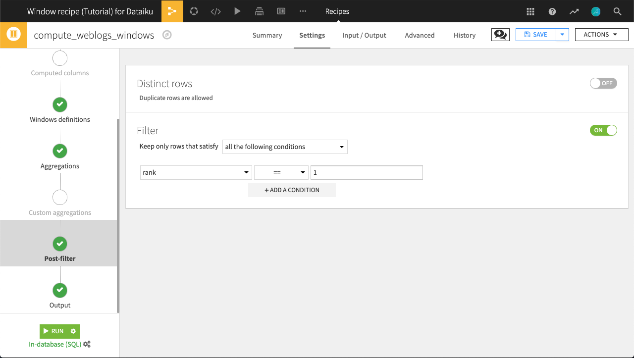
We want to only keep rows representing the first event of a session on any page, or where rank equals 1. We could achieve this with a Prepare recipe, but we can also utilize the Post-filter step of the Window recipe.

• Turn Filters On.

• Keep only rows where rank == 1.

Run the recipe. The output dataset now contains only events representing the first time that a user interacted with a page within a given session. Try verifying this outcome yourself with a Group recipe and a post-filter condition returning rows with count greater than 1.

Lead and Lag

Now we would like to know how much time was spent on each page in a session. Because in the previous step we identified the first event of a session on any page, we can compute the difference in timestamps to reveal how long a user spent on a particular page before navigating elsewhere.

Lag is the Window function for this job. Lag retrieves the value of a column in the previous (or a previous) row and inserts it in the current row in another column. Furthermore, DSS adds the Lagdiff function to automatically compute the difference between this previous value and the current value.

From the weblogs_windows dataset, where rank equals 1 for all rows, create a new Window recipe. Name the output dataset weblogs_lag. In the Windows definitions step:

• Partition columns by session_id

• Order columns by server_ts (ascending)

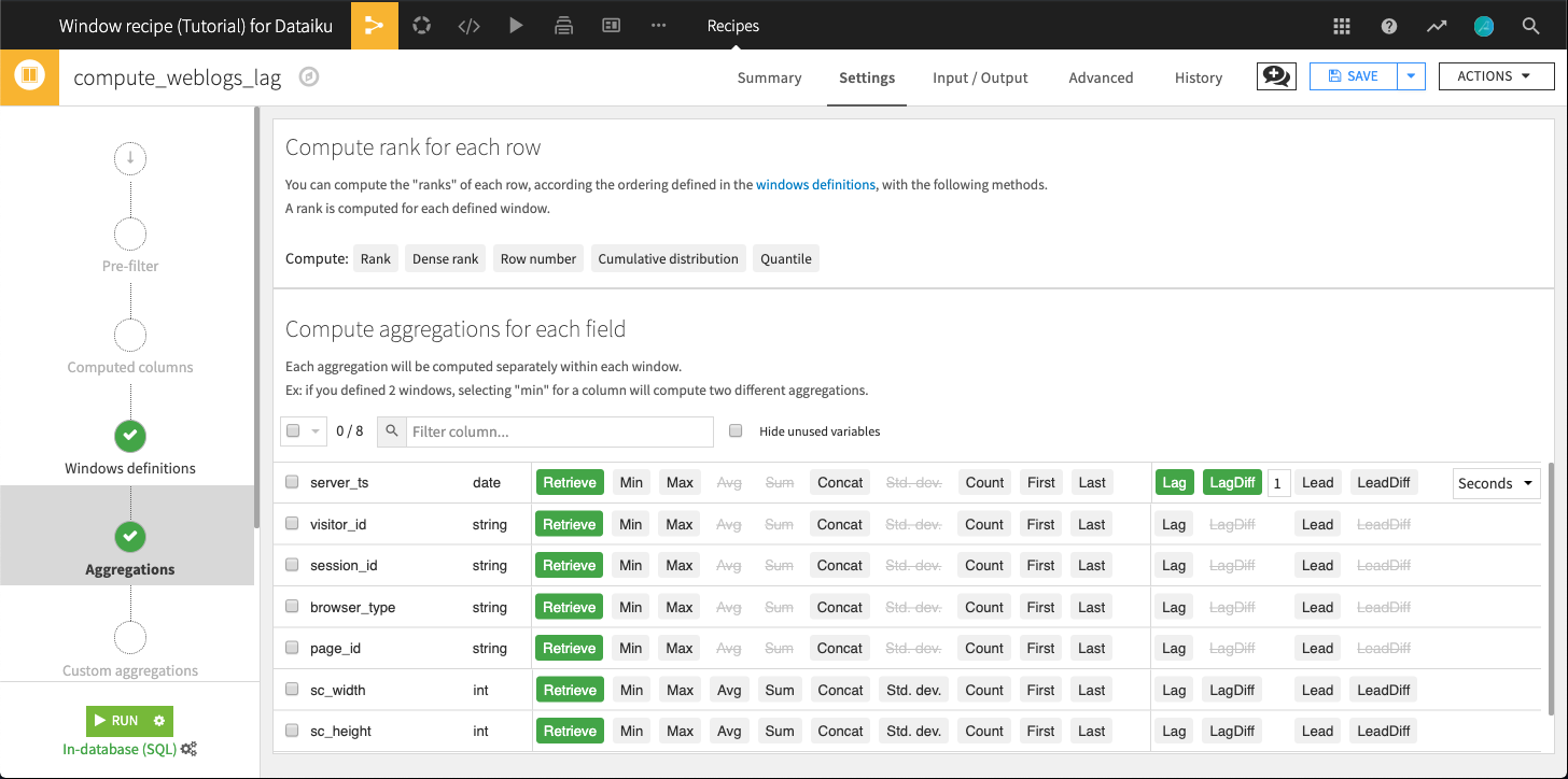
In the Aggregations step, choose to compute both Lag and LagDiff on the server_ts column.

• The “Lag offset” is 1 because we want to retrieve the value of the 1st previous row.

• For LagDiff, we also need to specify the unit in which the time difference will be expressed. Choose Seconds.

Run the recipe and let’s look at a few results in the output dataset.

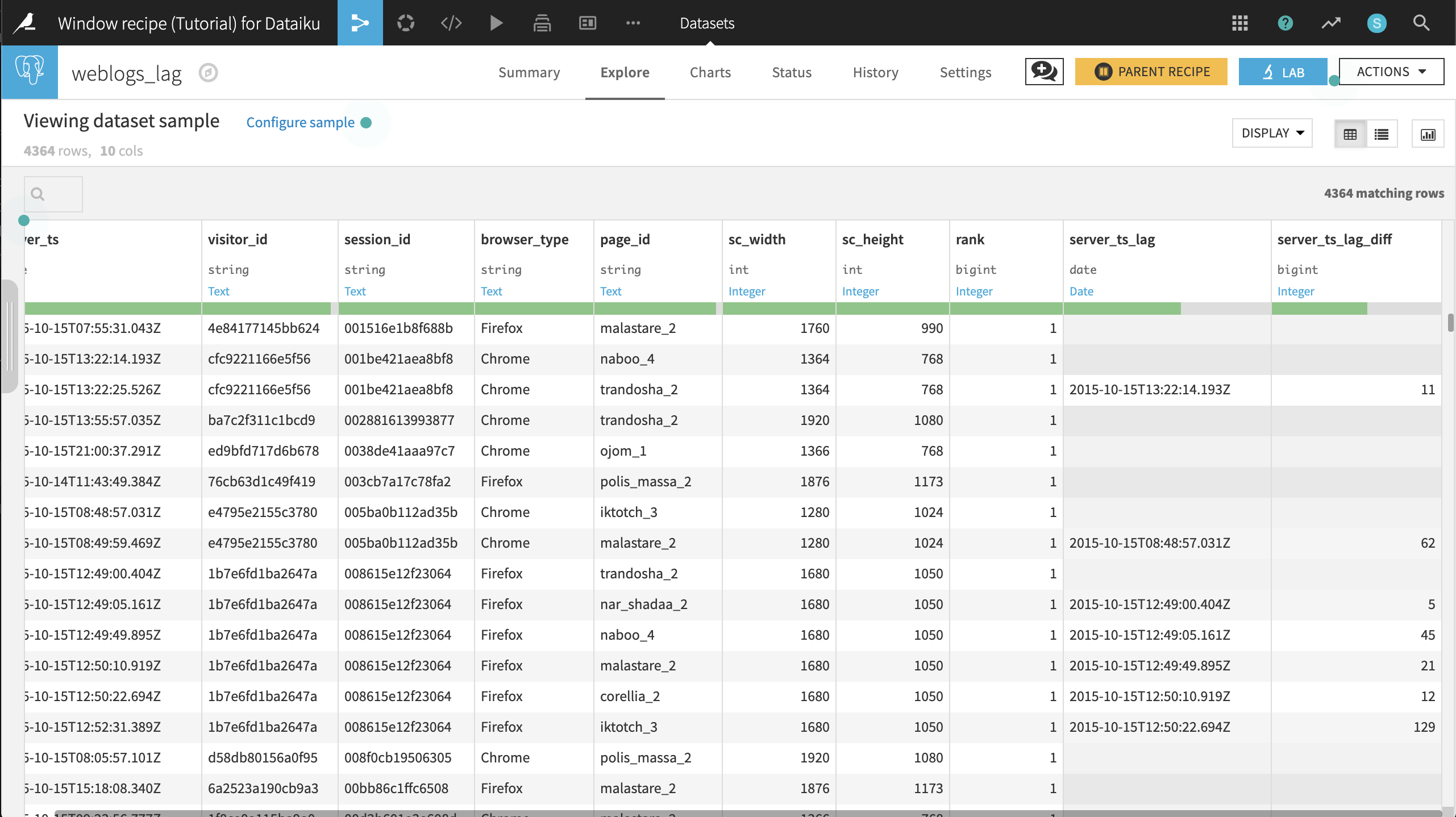
• Session 001516e1b8f688b only visited one page, malastare_2. There is therefore no information on how long they visited the page.

• Session 001be421aea8bf8 visited naboo_4 and trandosha_2. Here we see that the user spent 11 seconds on naboo_4.

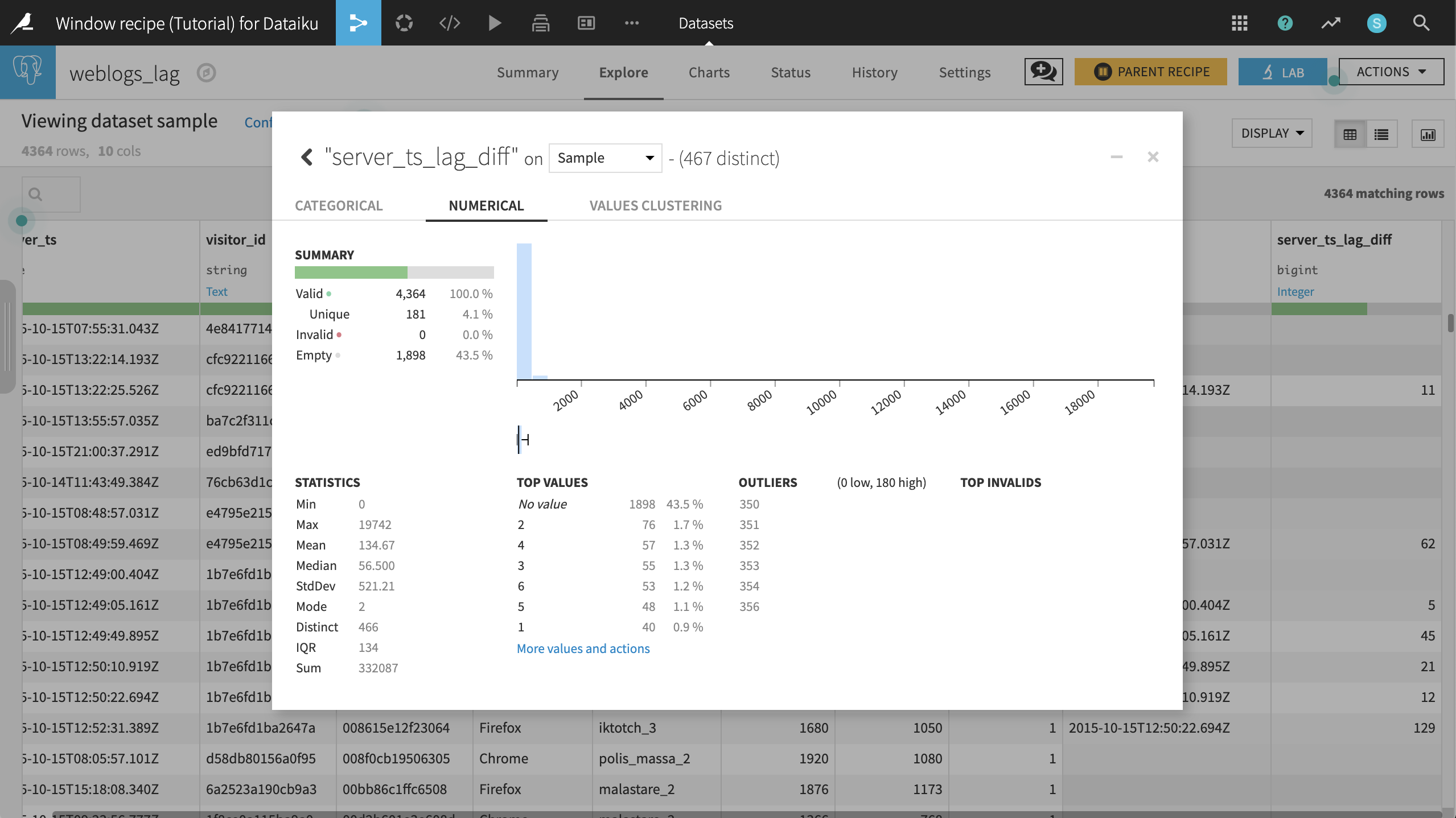
Opening the Analyze menu on the server_ts_lag_diff columns gives a few quick insights into the data. The maximum value is 19,742 seconds so that seems like a data error or some huge outliers. Even so, it looks like the distribution of page view times are highly right skewed, as we might expect.

What’s Next

The Window recipe opens a world of possibilities. As shown here, it can be used to add grouped calculations as a column, compute cumulative sums or moving averages, as well as leading and lagging differences.

To review, you can find a completed version of this Window recipe tutorial on the Dataiku gallery.