Concept: Window Recipe
In this lesson, let’s look at a powerful function for data enrichment, Windows. This lesson will cover:
a conceptual overview of the Window recipe;
and a practical demo of its advanced use in Dataiku DSS on credit card transactions data.
Note
If you are already familiar with the concept of Windows, you can skip to the practical demo or move to the hands-on tutorials.
A Window Cousin: The Group By Recipe
Before talking about Window recipes, let’s look at a related recipe, Group By.
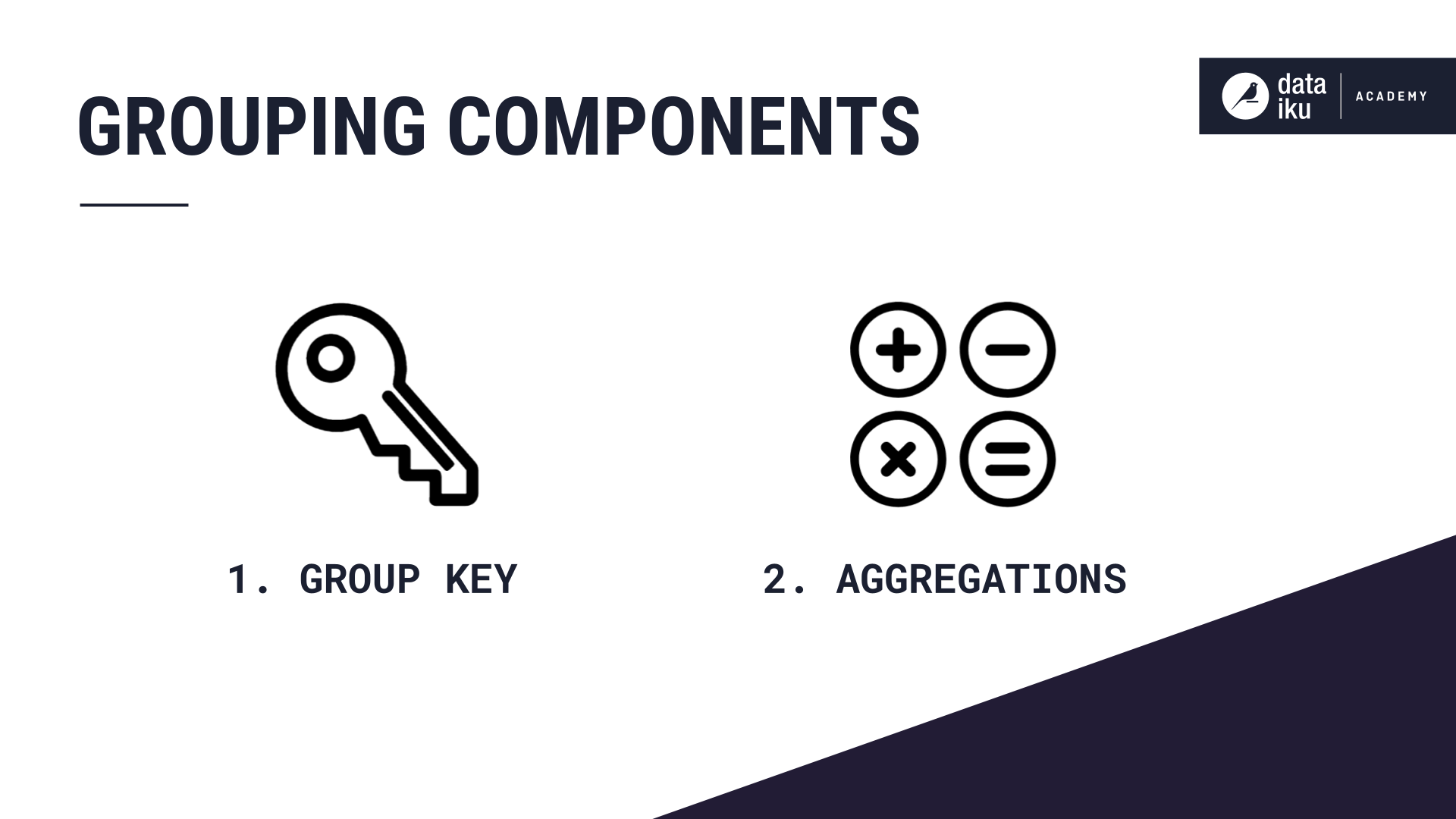
A Group by recipe has two important components: the Group Key and the Aggregations.
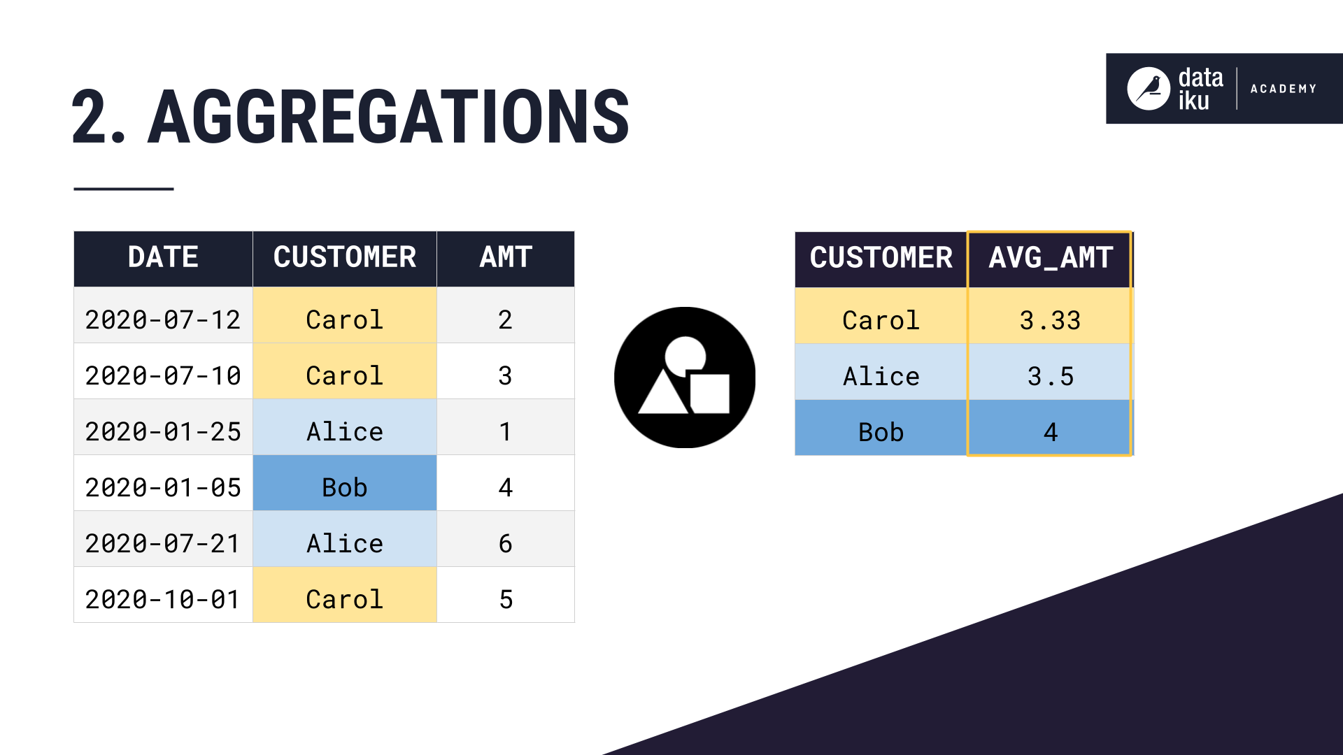
Let’s first take a customer orders dataset. Then, we choose a group key, in this case, Customer. And then choose to compute some aggregation, in this case the average amount of each order.
Notice the dimensionality of our dataset has changed. We have just one row per grouping key, rather than one row per order.
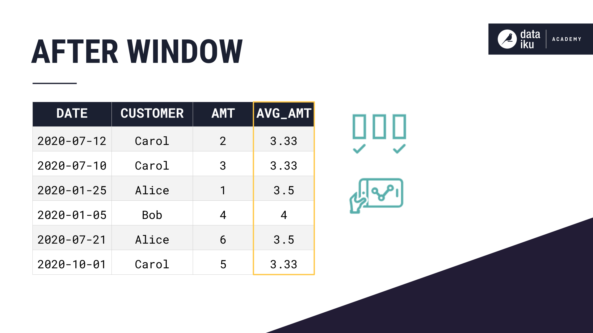
After Applying a Window
You may want to make these same grouped calculations on a dataset, while keeping the structure of the dataset the same. This is where we can use a window function.
A window function can perform this same grouped calculation, and append the values as a new column to the original dataset. This can help us make easy grouped comparisons or generate meaningful features for a machine learning model.
We can use a window to make calculations like:
Rank - is this a customer’s first order? second? third?
Lag - perhaps the quantity of each customer’s previous order.
A moving average can capture a customer’s average order quantity over the previous three days.
Window Components
A window function has two important components: the window definition and the aggregations.
These are similar to the components of a group by, with a few additions.
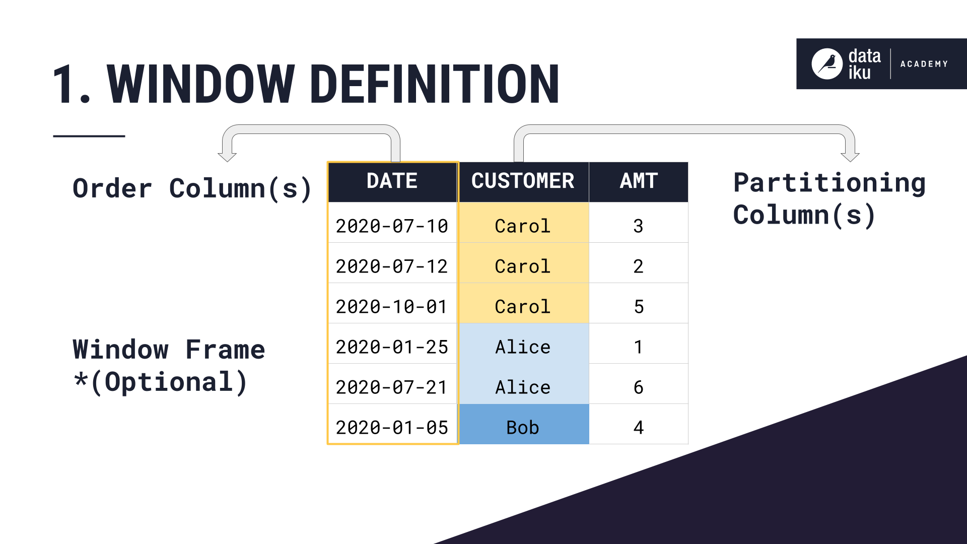
Window Definition
Let’s start with the window definition:
First, we choose the partition, or column to group by–in this case, the Customer.
Then, we order the rows within each partition by another column–in this case, by date, in descending order.
We can optionally define a window frame based on the ordering column, in this case, the date. This can limit our aggregation calculation to just a subset of rows within each partition.
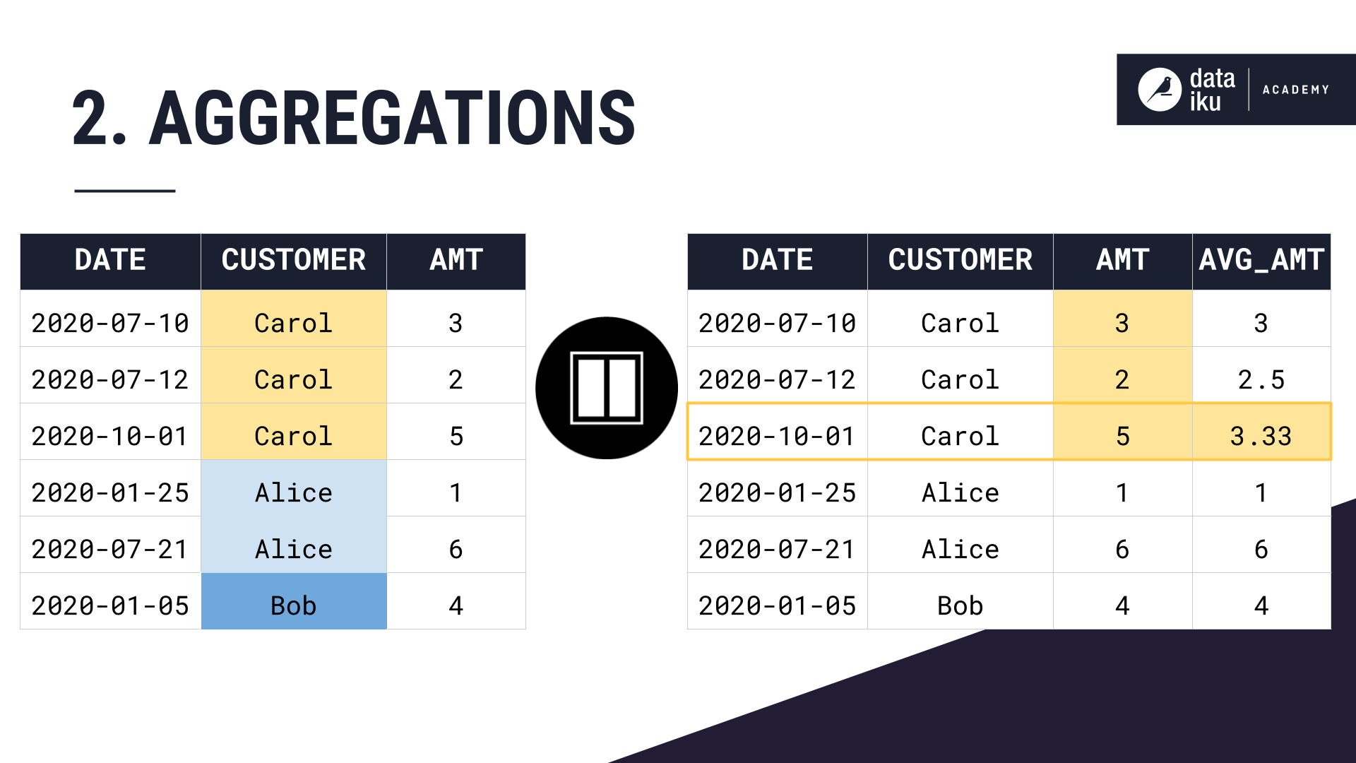
Window Aggregations
Now let’s look at the second component of a Window, the aggregations.
For each customer partition, ordered by date, and bounded by a window frame, what do you want to calculate?
Here, we chose to calculate the average amount–where the window definition was partition by customer, order by date, and no window frame. Remember, constricting the window frame is optional.
If we wanted to set a window frame which looks back at just the 3 previous months, and does not look at orders made in the future, our average amount calculation would look like this.
Let’s take a close look at why setting this window frame changes our column values.
We are partitioning our dataset by customer, ordering by date, setting a window frame of the previous 3 months till the current row’s date, and then computing an average amount over this window definition.
Same as before, we partition by customer, and order our rows within each partition by date.
Then we compute our average amount aggregation.
For Carol’s first purchase, she has no purchase history, so the rolling three-month average is just the current purchase amount, 3. For her second purchase, we can average the amounts from the current purchase and the previous purchase, as that one happened within the last three months. For her third purchase, we can average the amounts from all three of her purchases which all happened within the last three months.
Then with Alice’s first purchase, we restart our average calculation, just considering the current purchase amount. For Alice’s second purchase, we again restart our average calculation. Her first purchase happened more than 3 months ago, so we exclude it from the aggregation calculation.
Bob only has one purchase, so his rolling 3 month average amount is just 4.
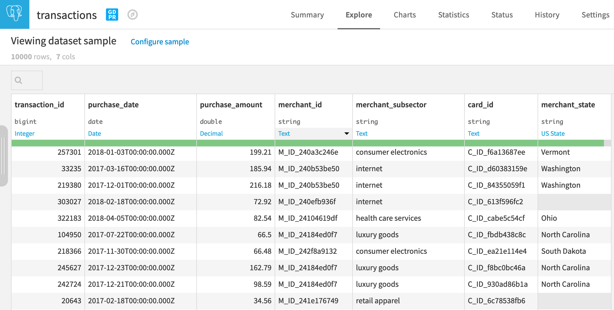
The Window Recipe in Dataiku
Now let’s take a closer look at how Windows work in Dataiku with some more realistic data.
We start with a dataset of credit card transactions. Notice that we have a timestamp for each transaction, a transaction ID, a purchase amount, a merchant, and a merchant subsector, among other information.
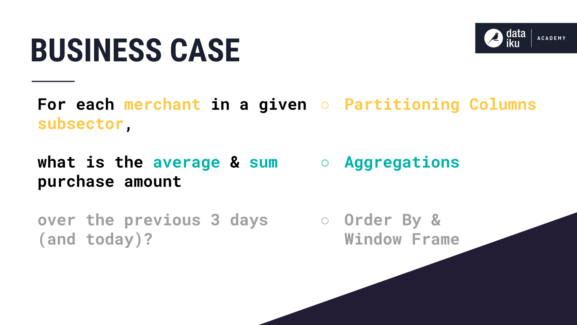
Here, we want to look at the average and the sum of purchase amounts for a given merchant subsector, as well as for each individual merchant. But imagine we want these aggregations to include only today and the previous 3 days.
At the same time, we want to keep each transaction in a separate row so that we can compare the individual purchase amount to the average for this merchant and this subsector.
This is a type of problem that the Window recipe is great for: keeping the structure of the data the same while getting some additional information by looking at similar rows.
Defining the Window
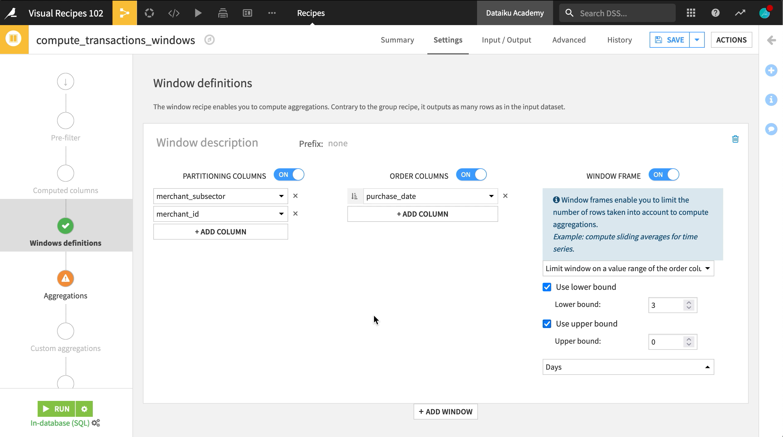
On the Window definition step, let’s turn on Partitioning and choose merchant_subsector, because we want to find the sum and average amount of transactions made to each merchant. Additionally, we also want to look at the sum and average purchase amount for each merchant ID in each subsector, so we can add a second partitioning column – merchant_id.
Then let’s order our rows within each partition by purchase_date in ascending order.
The third option–“Window Frame”– limits the number of rows your window can look at in each grouping. Let’s turn it on:
We have the option to limit the number of rows taken into account based on a value range from the order column, which in this case is the purchase date.
Let’s select this option and limit the rows to compute aggregations to only reflect the transactions made in the past 3 days, as well as the present day.
Choosing Aggregations
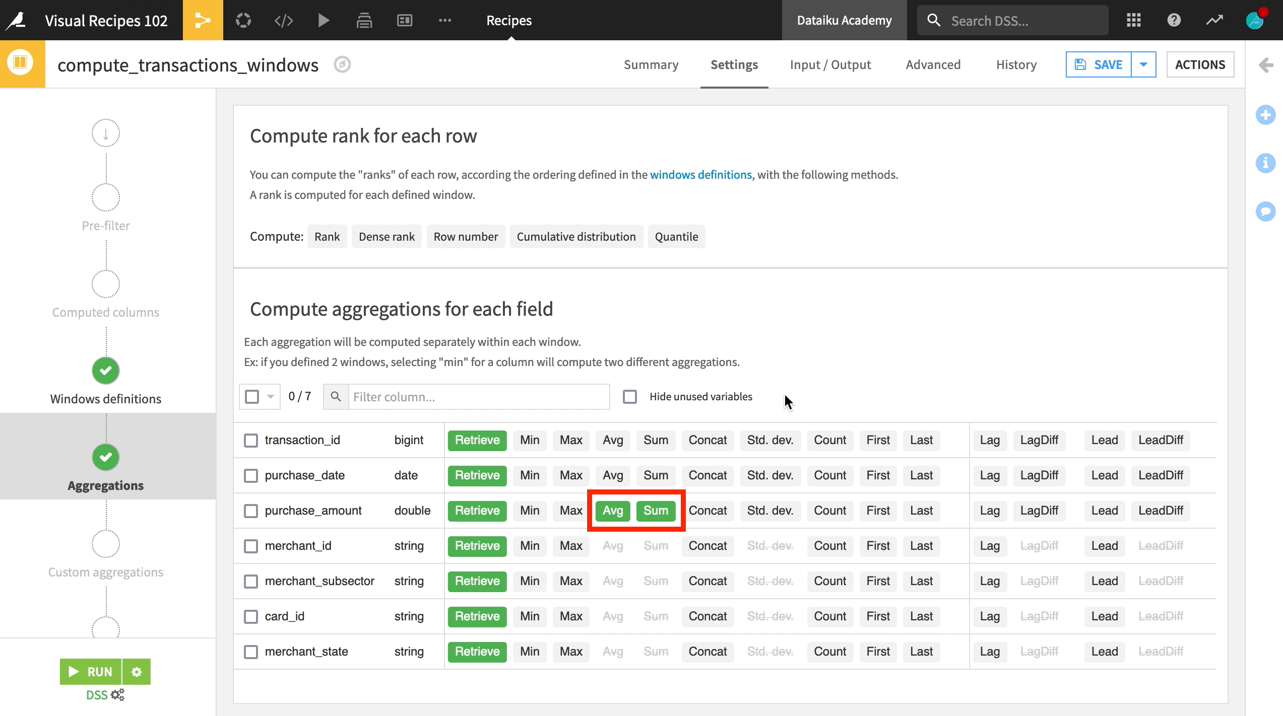
The Aggregations step lets you choose the aggregate metrics that our window will output for each grouping.
Here, we will choose the average, and sum of the purchase amount for each transaction, which will be aggregated by merchant and merchant subsector.
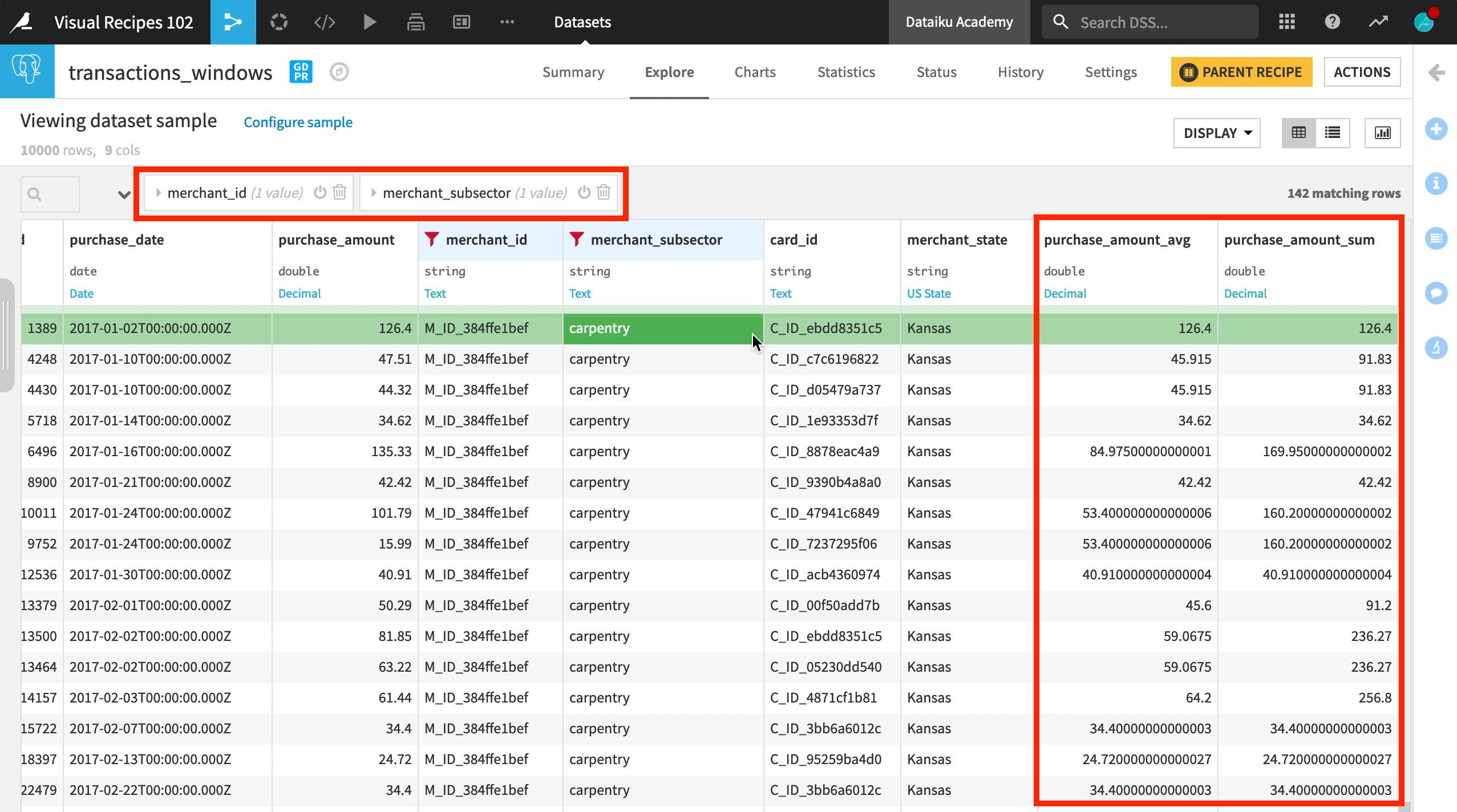
Interpret the Output
After running the recipe, we can see our new columns in the output dataset: purchase_amount_avg and purchase_amount_sum
We can now filter by merchant ID and subsector to see the average and sum of purchases for this grouping within the defined window frame of the past three days.