Prepare the Bike Stations Dataset

The first dataset provides a map of the bike station network.

• In the Flow, select + Recipe > Visual > Download.

• Name the output folder bikeStations and create the recipe.

• Add a new source and specify the following URL: http://capitalbikeshare.com/data/stations/bikeStations.xml.

• Run the recipe to download the files.

Note

As this data comes directly from Capital Bike Share, the exact number of rows in your dataset may differ slightly from the project displayed in the Gallery. While this should not have an impact on the overall results, do be aware that your own results may not be exactly the same.

Having downloaded the raw data, let’s now read it into Dataiku DSS by creating a Files in Folder dataset.

• From the bikeStations folder, click on Actions > Create a dataset (found in the upper-right corner).

• Click Test to let Dataiku detect the XML format and parse the data accordingly.

• Accept the dataset name bikeStations and create it.

In the new dataset, go to the Lab and create a new Visual Analysis. Accept the default name, and add the following steps to the script:

• In order to geographically map the bike stations, we need to create a GeoPoint from the latitude and longitude of each station. Notice, however, that a small number of bike stations have extraordinarily precise geographic coordinates. A quick Google search suggests that six decimal places gets you to within 11 cm! So entries with coordinates to 14 decimal places surely seem like an error.

• Let’s round these extraordinarily precise values to a more reasonable level without adding any unwarranted precision to other values.

  • Using the Copy columns processor, copy the long column into a new column, long_round.

  • Round the long_round column to 6 decimal places using the Round numbers processor.

  • With a Formula, redefine the column long with the expression if (length(long) > 10, long_round, long).

  • Select these three steps and move them into a Group called Fix lon/lat data.

  • Copy and paste the steps within the group just created. Change instances of long to lat. The group should have a total of 6 steps.

• Now we can create GeoPoints from the clean lat and long columns.

  • Use the Create GeoPoint processor with the lat and long columns as the inputs and geopoint as the output column.

• Delete 13 columns we won’t use. This means removing all columns except for nbBikes, long, name, lat, and geopoint.

• Rename the column name to the more-specific station_name to avoid naming conflicts later.

Switch to the Charts tab and create a new Scatter Map:

• Use geopoint as the “Geo” column.

• Use nbBikes as the “Details” column to color the bubbles.

• To make the stations with the most bikes more visible, change the palette color to “Green-red” from the Color dropdown menu.

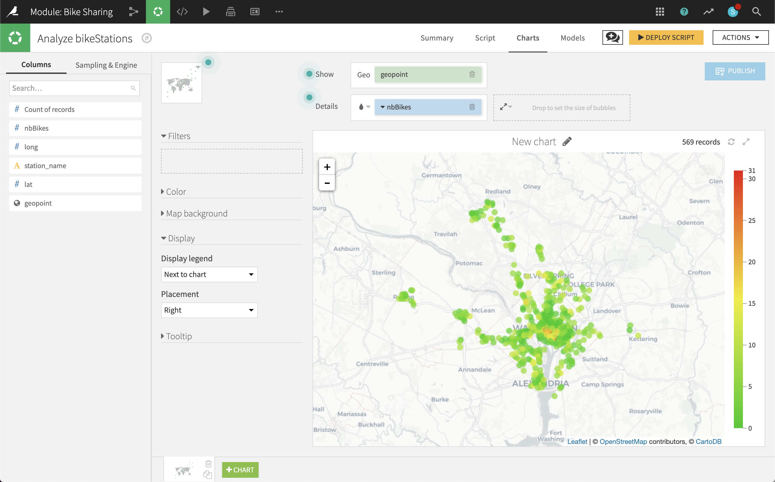
At first glance, it appears that a very small number of stations in central DC have a large number of bikes, while a much larger number of surrounding stations have very few bikes (even 0).

Deploy the Visual Analysis script, accepting the default output name, bikeStations_prepared. Check the boxes to create charts on the new dataset and build it now.

We now have a clean dataset of the geographic locations of all bike stations and the number of bikes they hold.