Hands-On: Extrema Extraction

In the previous hands-on lesson on the time series Windowing recipe, we demonstrated how to build a wide variety of causal and non-causal window aggregations, adjusting parameters like width, bounds, and shape along the way.

The Extrema Extraction recipe finds a global extremum (minimum or maximum) in one dimension of a time series and performs windowing functions around the timestamp of the extremum on all dimensions.

Getting Started

This hands-on lesson picks up where the Windowing hands-on lesson finished. If you have not completed that lesson, you only need to have completed the Resampling hands-on lesson so that you have the orders_resampled dataset in your Flow.

Compute Aggregates around the Global Maximum

Let’s use the Extrema Extraction recipe to find the global maximum amount spent for each time series, and then compute the average spent in a 7-day non-causal (bilateral) window around each global maximum value.

• Click the orders_resampled dataset and then the Time Series Preparation plugin in the right panel.

• Select the Time series extrema extraction recipe from the dialog that appears.

• Name the output dataset extremum. Then create the output dataset.

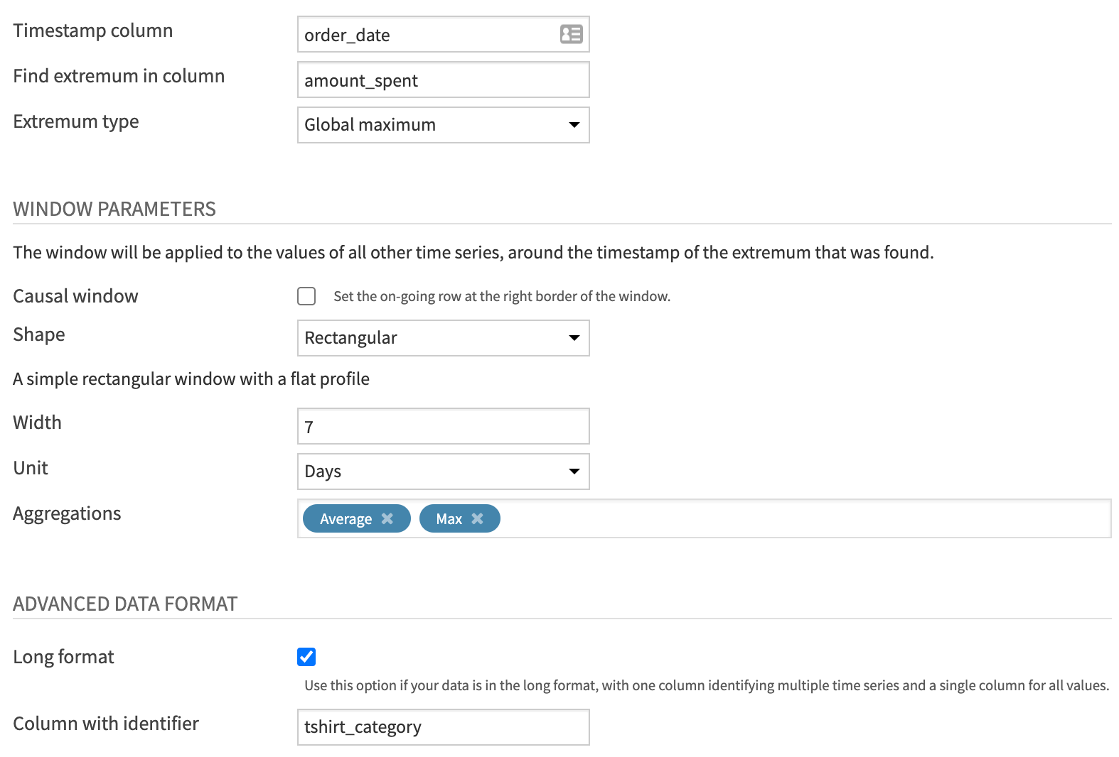
In the recipe dialog, specify the following parameters:

• Set the value of the “Time column” to order_date.

• Set “Find extremum in column” to amount_spent.

• Specify the “Extremum type” as Global maximum.

For the Window parameters:

• Leave the “Causal window” box unchecked to use a non-causal window (that is, a window which places the timestamp for the extremum point at its center).

• Specify a Rectangular shaped window of 7 Days.

• Select two aggregations: Average and, for the purpose of checking our result, Max.

Finally, as before, check the “Long format” box and specify tshirt_category as the value for the “Column with identifier” parameter.

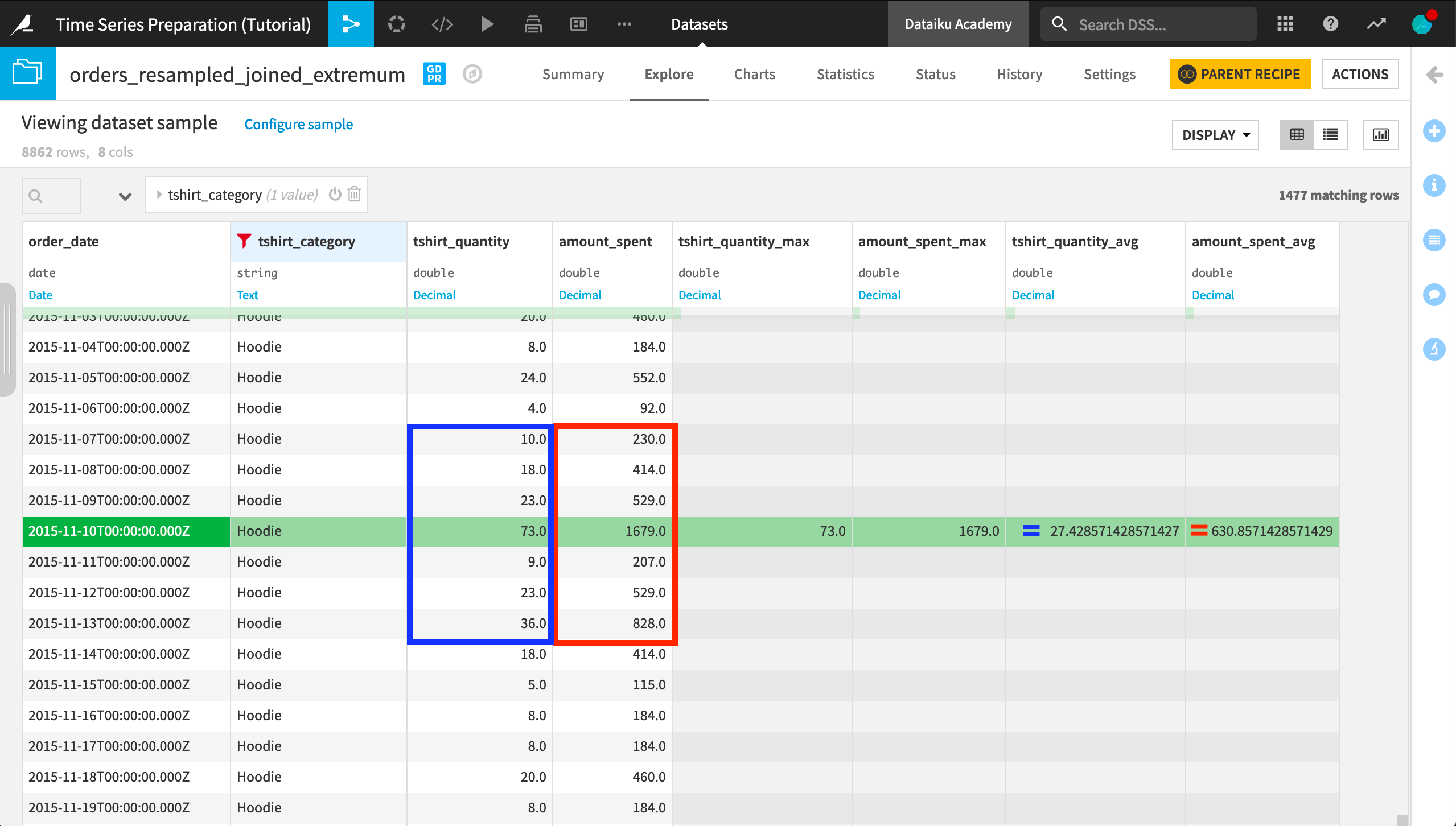
After building the output dataset, we have four new columns because we started with two dimensions (amount_spent and tshirt_quantity) and requested 2 aggregations.

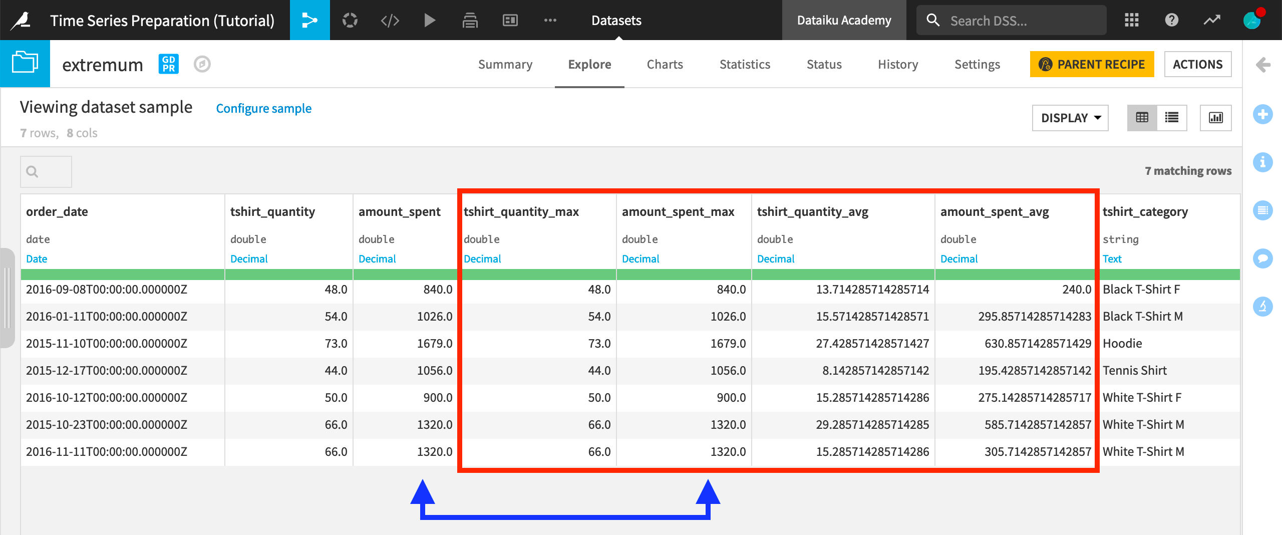
The amount_spent_max column should be exactly the same as the amount_spent column because we are building the window frame around the global maximum of the amount_spent column for each time series.

Reading this output, we can see that the average amount spent in the seven days around the global maximum (of the amount_spent) for each time series is considerably lower than the global maximum value. For example, the maximum amount_spent on “Hoodies” was $1679, but in the seven days surrounding the date of this spending, the average spent on hoodies was only about $630.

Also, notice that the output dataset consists of only one row for each time series in the orders_resampled dataset. The only exception is for ties among the selected global extremum. Here, there is a tie among the highest amount_spent on the “White T-Shirt M” time series, and so aggregations are returned for both “2015-10-23” and “2016-11-11”.

Verify Aggregates with a Join

The result of the Extrema Extraction recipe conceals the values that were aggregated in the window frame.

We could reveal these values by joining the extremum dataset back into the resampled data.

• Select the orders_resampled dataset and create a Join recipe.

• Add extremum as the second input dataset.

• Name the output dataset orders_resampled_joined_extremum and create the recipe.

• Run the recipe.

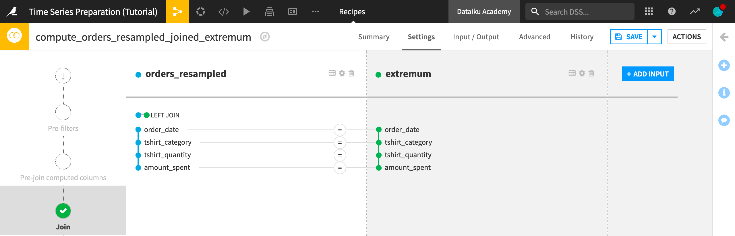
In the output dataset, we have four new aggregation columns alongside the original orders data. To find the correct part of the time series,

• Filter one of the aggregations columns for OK values.

• Filter for one tshirt_category, such as “Hoodie”.

• Make note of the order_date (“2015-11-10”).

• Remove the filter for OK values and scroll to the order_date.

If we take this row for example, we can see the exact values that produced the window aggregate values.

Compute Aggregates around the Global Minimum

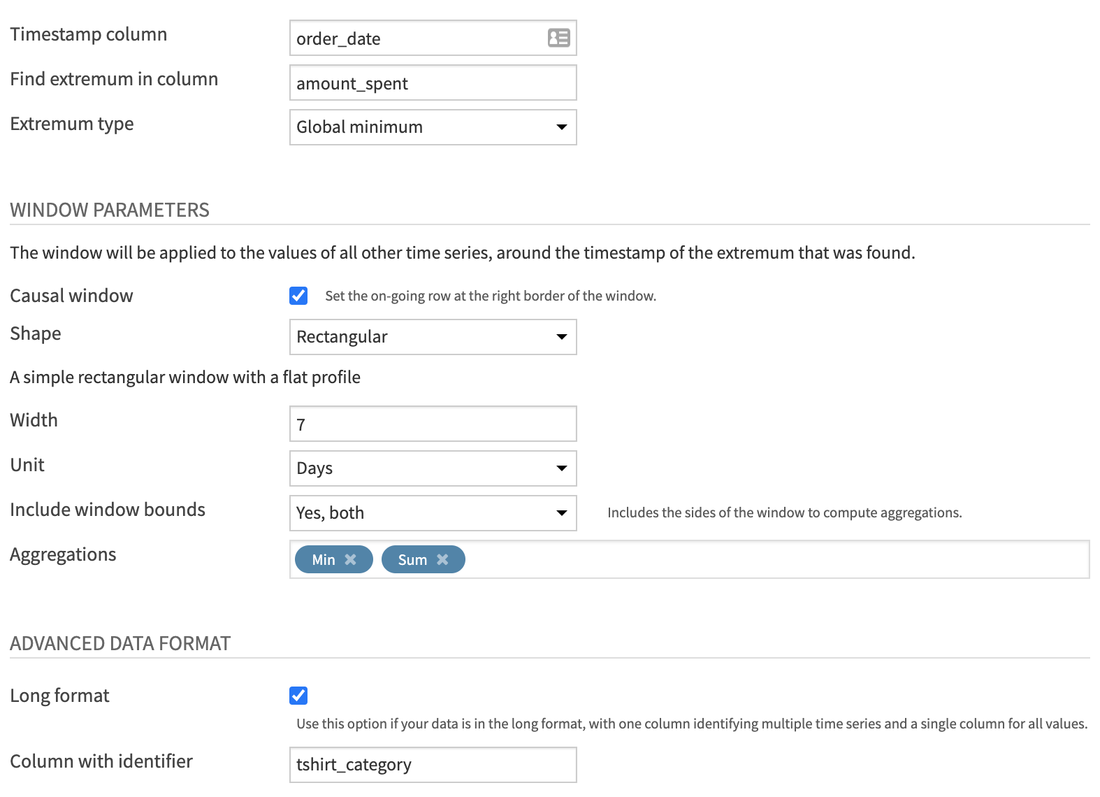
For some more practice, let’s build a window frame around the global minimum.

• Return to the compute_extremum recipe.

• Change the “Extremum type” from Global maximum to Global minimum.

• This time, build a Causal window of 7 days including both bounds.

• In terms of aggregations, change the Max to a Min and Average to a Sum.

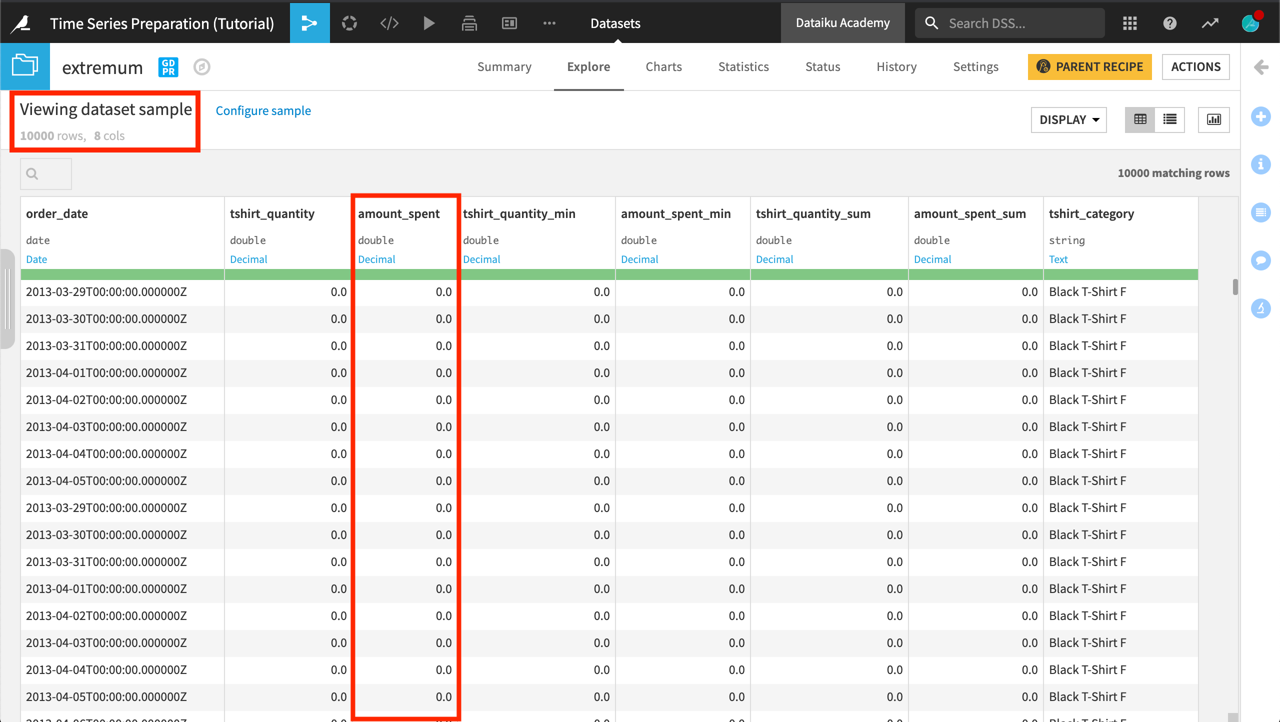
After running the recipe, the output has way more than one row per time series! This is because many rows in a time series share the same global minimum of 0. If there is a tie for extremum value in a time series, the recipe returns all rows sharing the global extremum.

What’s next?

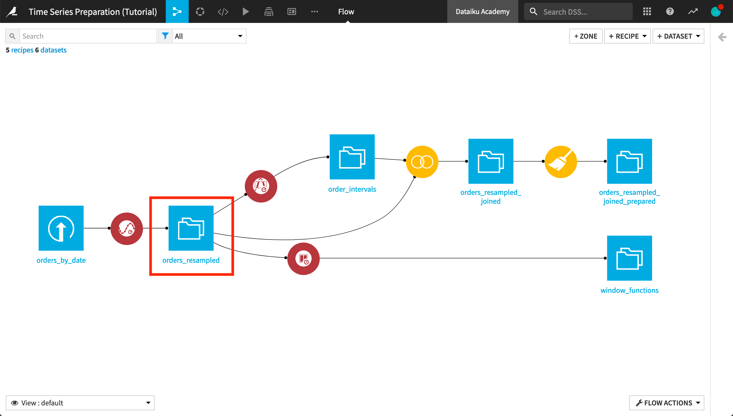
Congratulations! If you have followed along with all of the hands-on lessons, your final Flow should resemble the image below.

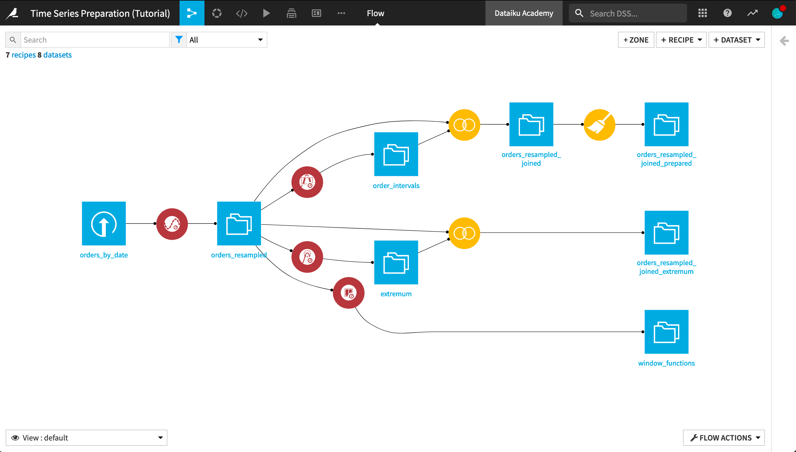
At this point you have gained experience using each one of the four recipes in the Time Series Preparation plugin.

With prepared time series data, you’ll be ready to model and forecast your time series data.