Hands-On: Time Series Windowing
For noisy time series data, observing the variations between successive time series values may not always provide insightful information. In such cases, it can be useful to filter or compute aggregations over a rolling window of timestamps.
In this hands-on lesson, we’ll build a wide variety of possible window aggregations using the Time series windowing recipe in the Time Series Preparation plugin.
Getting Started
This hands-on lesson picks up where the Interval Extraction hands-on lesson finished. If you have not completed that lesson, you only need to have completed the Resampling hands-on lesson so that you have the orders_resampled dataset in your Flow.
Note
This tutorial focuses primarily on usage of this recipe. For a more detailed walkthrough of the parameters, please refer to the previous concept videos or text summary lessons.
Causal Windows
Let’s start with a simple causal, rectangular window frame — the kind that can be easily built using the visual Window recipe.
From the orders_resampled dataset:
Apply the Time series windowing recipe from the Time Series Preparation plugin.
Name the output dataset
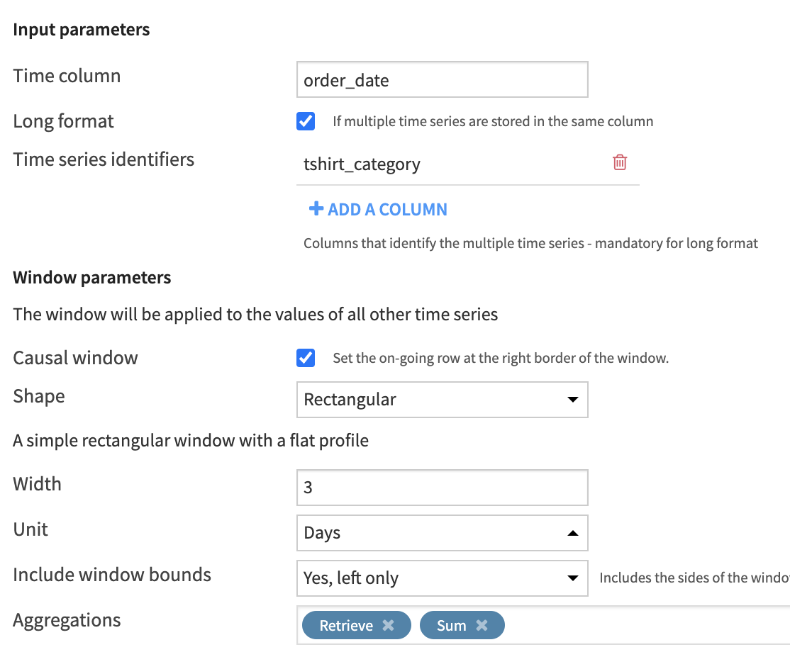
window_functions. Then create the output dataset.Set the value of the “Time column” to
order_date.Keep the “Causal window” box checked and the default shape Rectangular.
Define the size of the window frame by specifying a value of
3for the “Width” and Days as the “Unit”.Set “Include window bounds” to Yes, left only to use a strictly causal window that does not include the present observation.
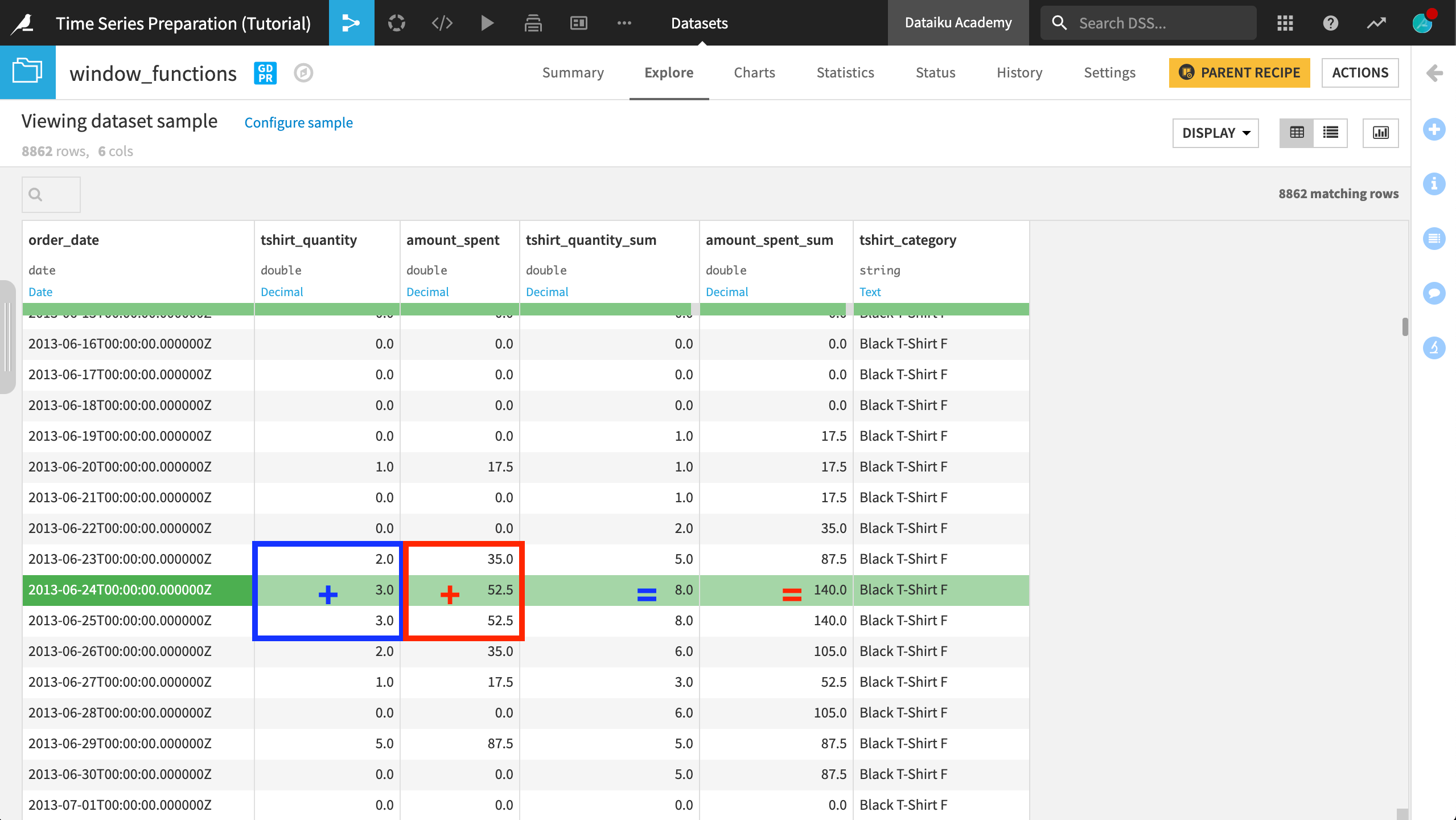
In terms of “Aggregations”, choose Retrieve to return the time series values for each day and Sum to compute the rolling sum.
As before, check the “Long format” box and supply tshirt_category as the identifier column.
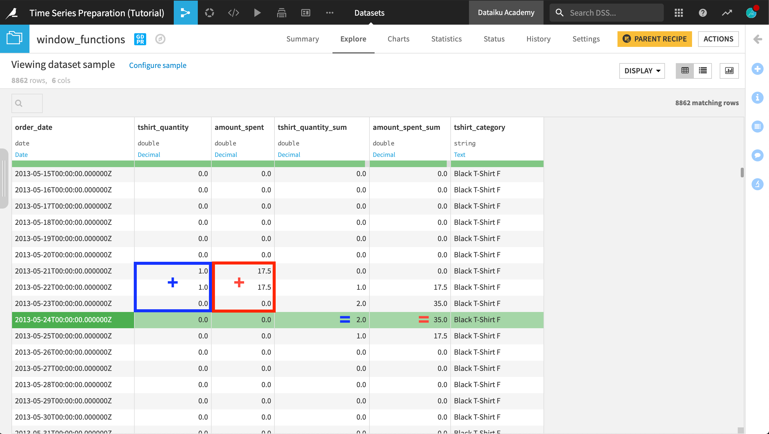
After running the recipe, scroll through the output dataset and verify the output is what you expected.
Tip
On your own, adjust the window parameters one at a time and verify the result is what you expect. For example, increase the width of the window frame; include or exclude the bounds.
Non-Causal Windows
Now let’s switch to a non-causal or bilateral window, where the current row will be the midpoint of the window frame instead of the right border.
Return to the compute_window_functions recipe.
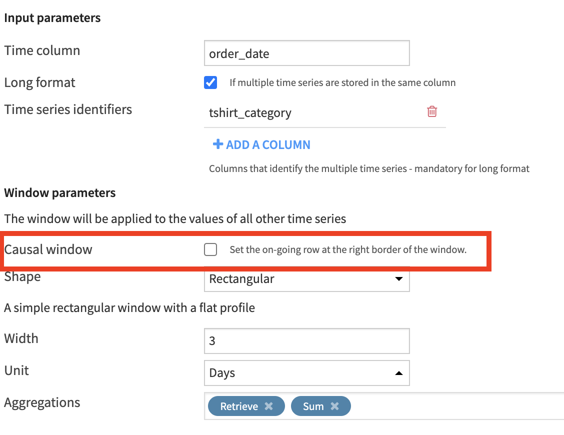
Uncheck the “Causal window” box to define a non-causal window.
Keep all other parameters the same and run the recipe.
Scrolling through the output, we can see how past, current, and future values are included in the window frame for any given row.
Tip
Verify for yourself what values are included in a non-causal window frame of even width.
Changing Units
Even though our data is recorded at a daily interval, the recipe allows us to specify other units.
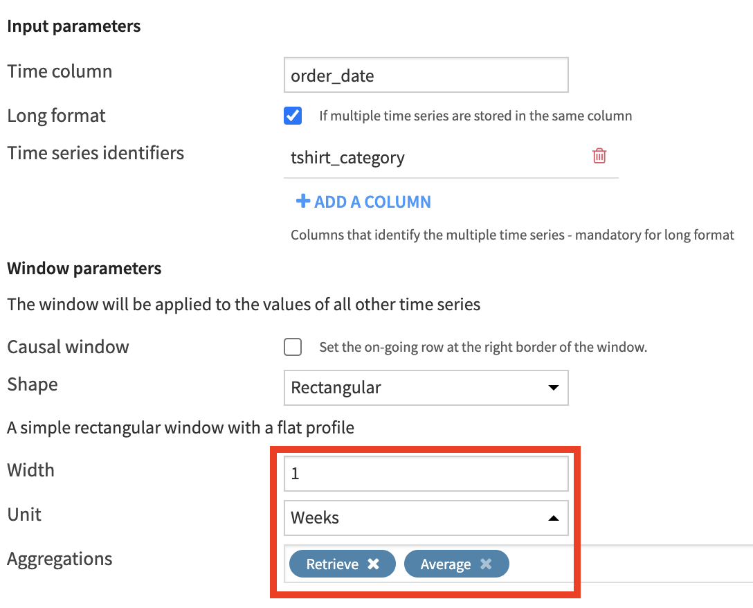
Return to the compute_window_functions recipe again.
Change the window size from 3 Days to 1 Week.
Change the Aggregations from Retrieve and Sum to Retrieve and Average.
Keep all other parameters the same and run the recipe.
In the output dataset, we can now see 7 days included in the rolling averages for the tshirt_quantity and amount_spent columns.
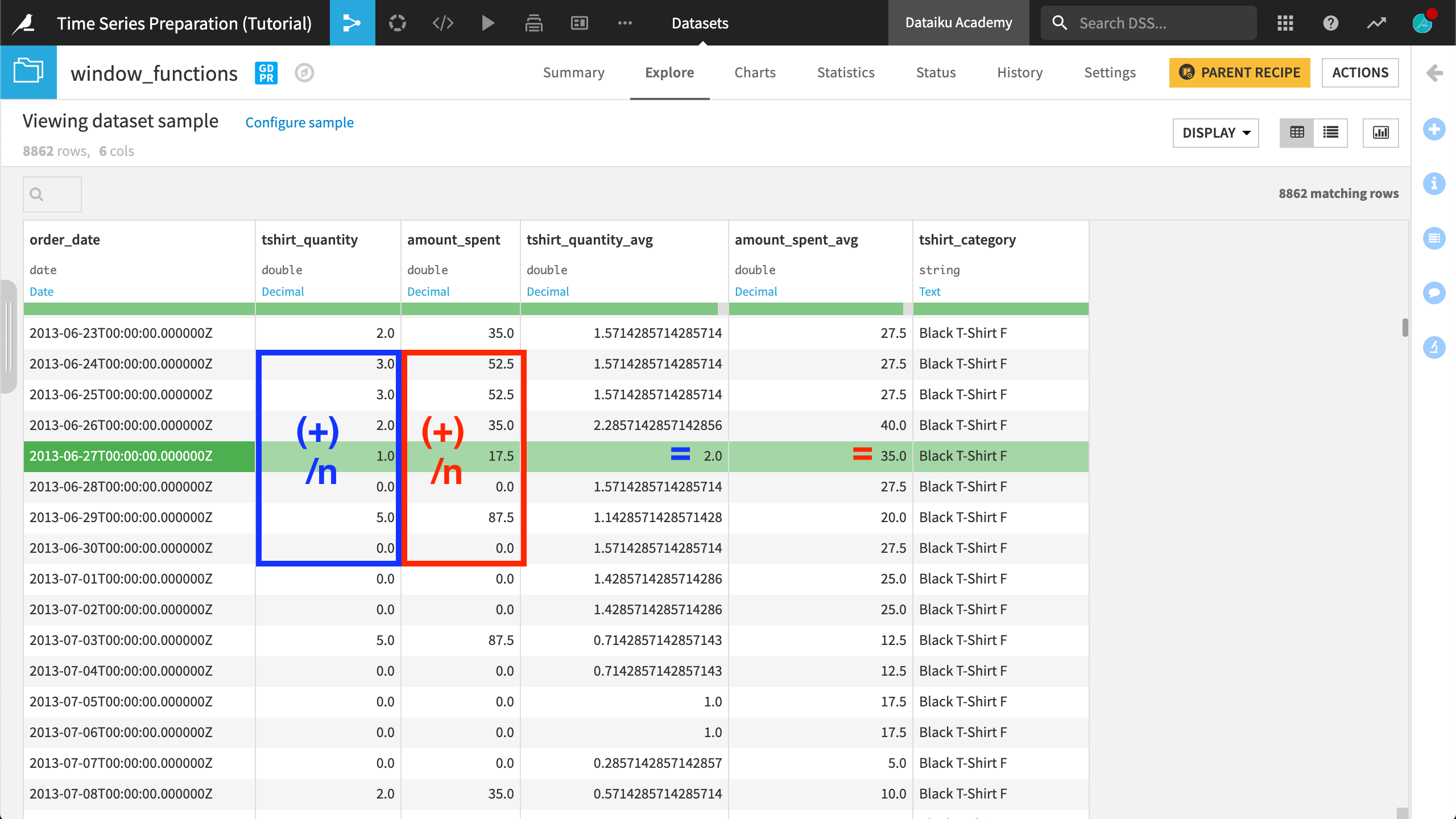
With a plot on the aggregation column, you can verify the smoothing effect on the data.
Tip
Verify on your own if there is a difference between a 7 day and a 1 week window frame.
Triangle Windows
All of the window frames we have built thus far have been rectangular in shape. Now let’s try a triangle.
Return to the compute_window_functions recipe once more.
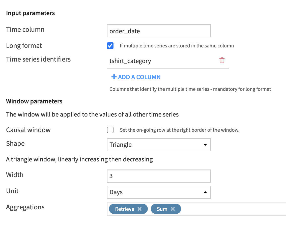
Change the Shape parameter from the default Rectangular to Triangle.
Reduce the size of the window frame from 1 week to 3 Days.
Change the Average aggregation back to a Sum.
Note
The only difference between this example and the first non-causal (bilateral) window example is the shape parameter.
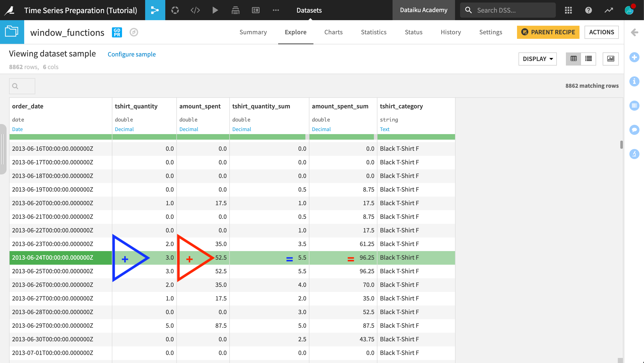
For “2013-06-24”, the moving sum of amount_spent is “96.25” using a triangular window, whereas that same sum was “140” using a rectangular window. That is because a triangular window of this width assigns a weight of 0.5 to the first and last row of the window frame and 1 to the center row.
Tip
On your own, observe changes in the output when using non-linear window shapes.
Next Steps
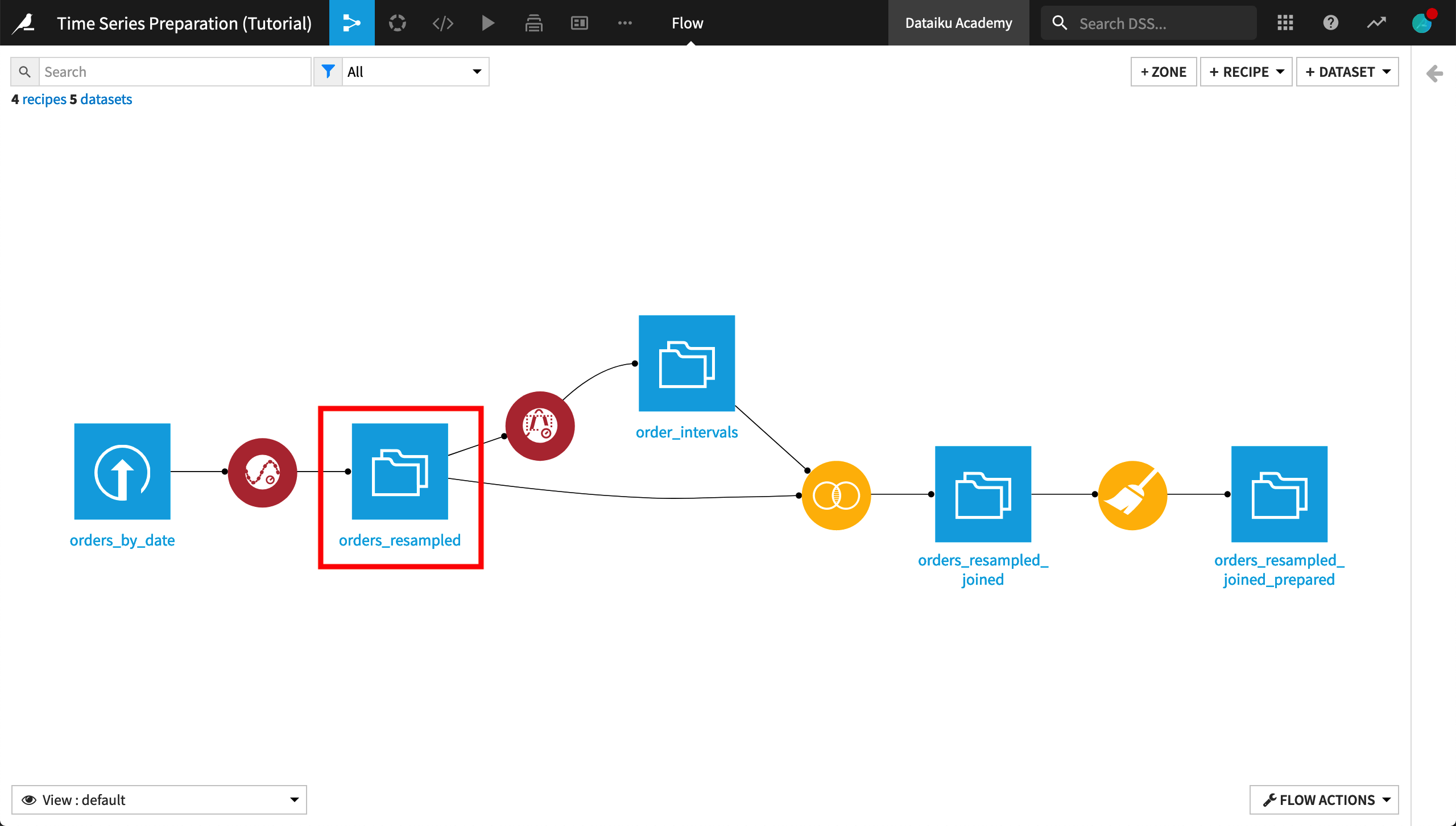
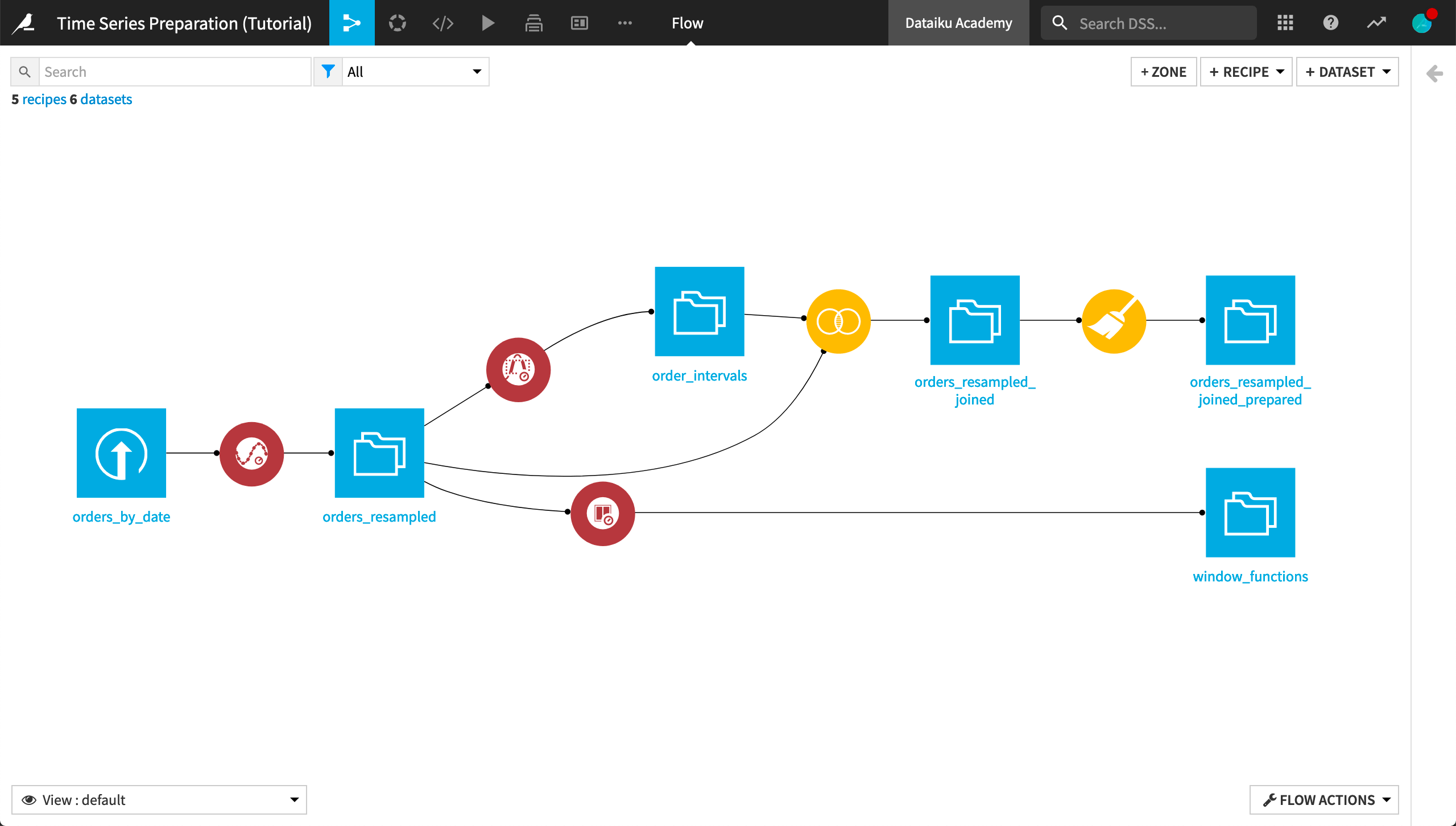
Congratulations! Your final Flow should resemble the image below.
You are now comfortable building a wide variety of window frames over time series data.
In the next section of this course, you’ll apply your knowledge of defining window frames to finding aggregates around global extrema values of time series.