Concept Summary: Time Series Interval Extraction Pt 3

After having explored the motivation and mechanics of the Interval Extraction recipe from the Time Series Preparation plugin in Parts 1 and 2, let’s finally test out how it works in Dataiku DSS in Part 3.

Using the Interval Extraction Recipe in Dataiku DSS

Note

This video lesson accompanies the explanation found below.

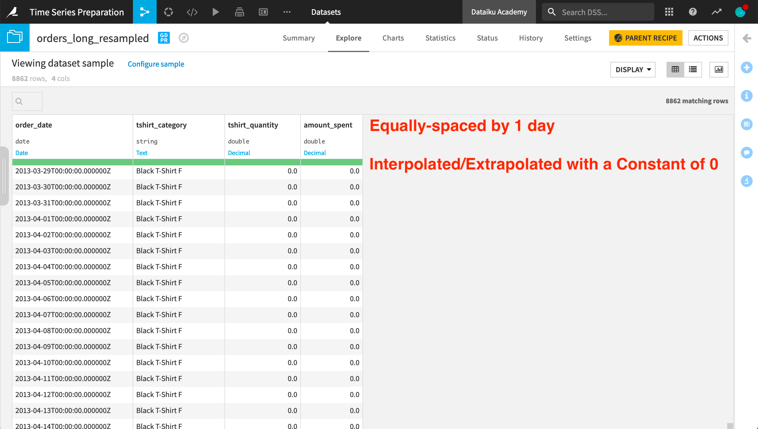
In the Resampling demo video, we used the Resampling recipe to equally space and interpolate the wide version of the orders data. Having multiple independent time series (one for each product category), we’ll have to work with the data in long format to apply the Interval Extraction recipe.

It is not required, but it is often advisable to first resample the data to make sure we understand the nature and meaning of any gaps in the time series. For this reason, we’ll apply the Interval Extraction recipe to the long format version of the resampled orders dataset.

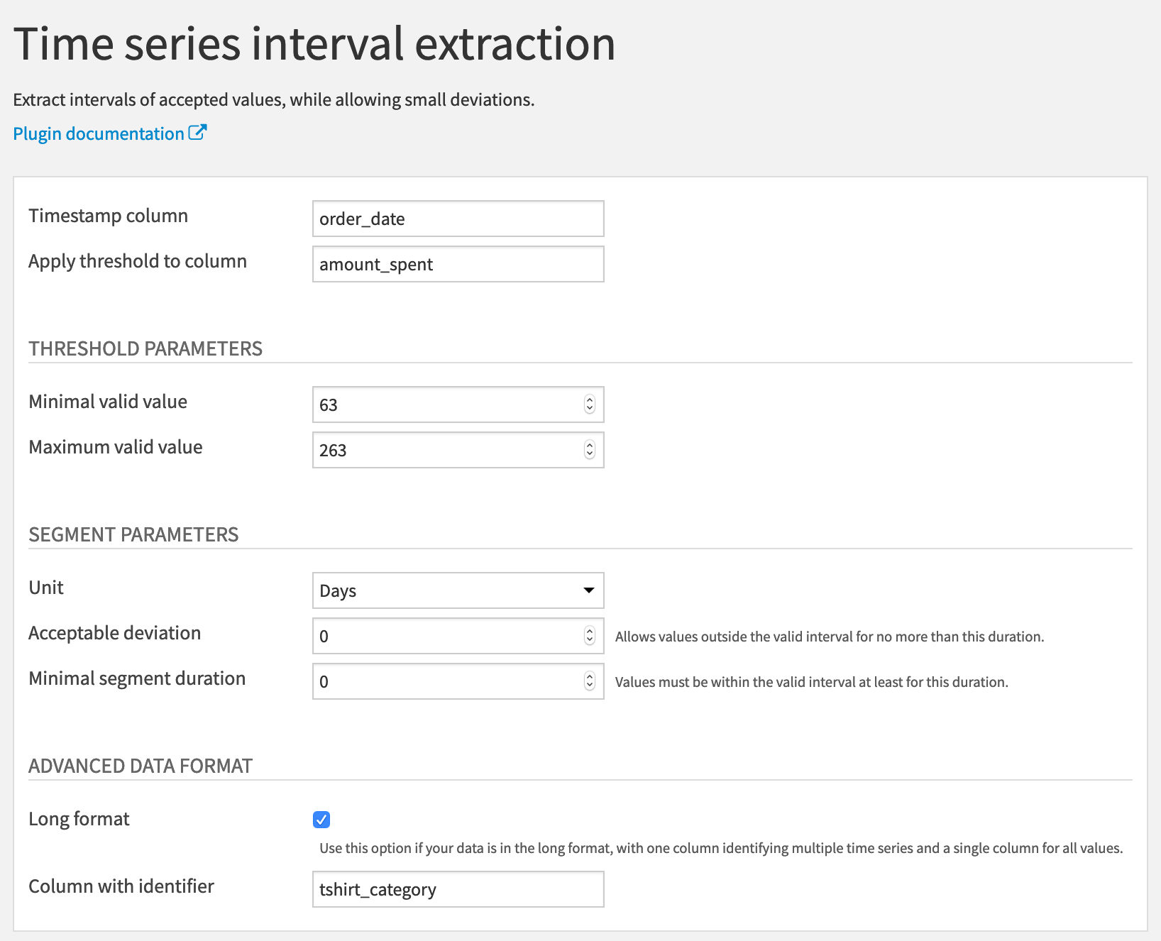
In the recipe dialog, we must provide a parsed date column as the value for the timestamp column. We also need to specify one numerical column to which the threshold range will be applied. Here we will use the amount_spent column.

We then need to define the lower and upper bounds of the threshold range. If we return to the input data, using the Analyze tool on the amount_spent column, we can gain some quick insights into the distribution.

For the whole dataset, the mean is about 163 with a very large standard deviation. For this example, we’ll set the minimal valid value at 63 and the maximum valid value at 263– 100 above and below the mean.

For now, let’s keep the acceptable deviation and the minimal segment duration both at 0 days.

Finally, we know this data is in long format, identified by the tshirt_category column.

In the output, we have the original four columns, plus one new column, “interval_id”. For each independent time series in the dataset, the recipe starts assigning interval IDs from 0 and increases from there.

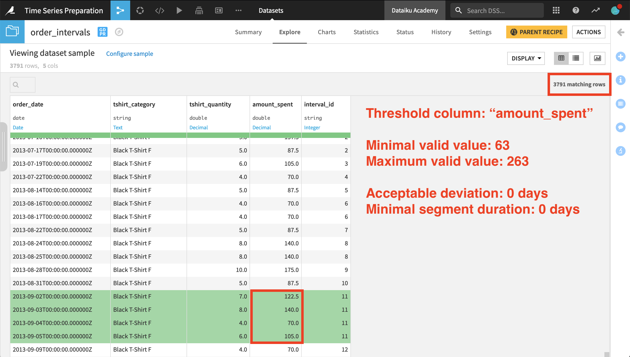
Several of the first few intervals have only a single timestamp belonging to them. For the 11th interval ID, however, we have four consecutive days with a value for amount_spent within the threshold range.

We should also note that only about 40% of the original rows remain when we perform interval extraction. The others do not meet the required criteria to be assigned an interval ID.

Note

If we were to look at another product category (a separate time series), the interval IDs reset to 0, and this time series has its own sequence of interval IDs. This suggests that an interval ID, such as 6, for one product category is not related to an interval ID for another category, because the categories represent different time series in the dataset.

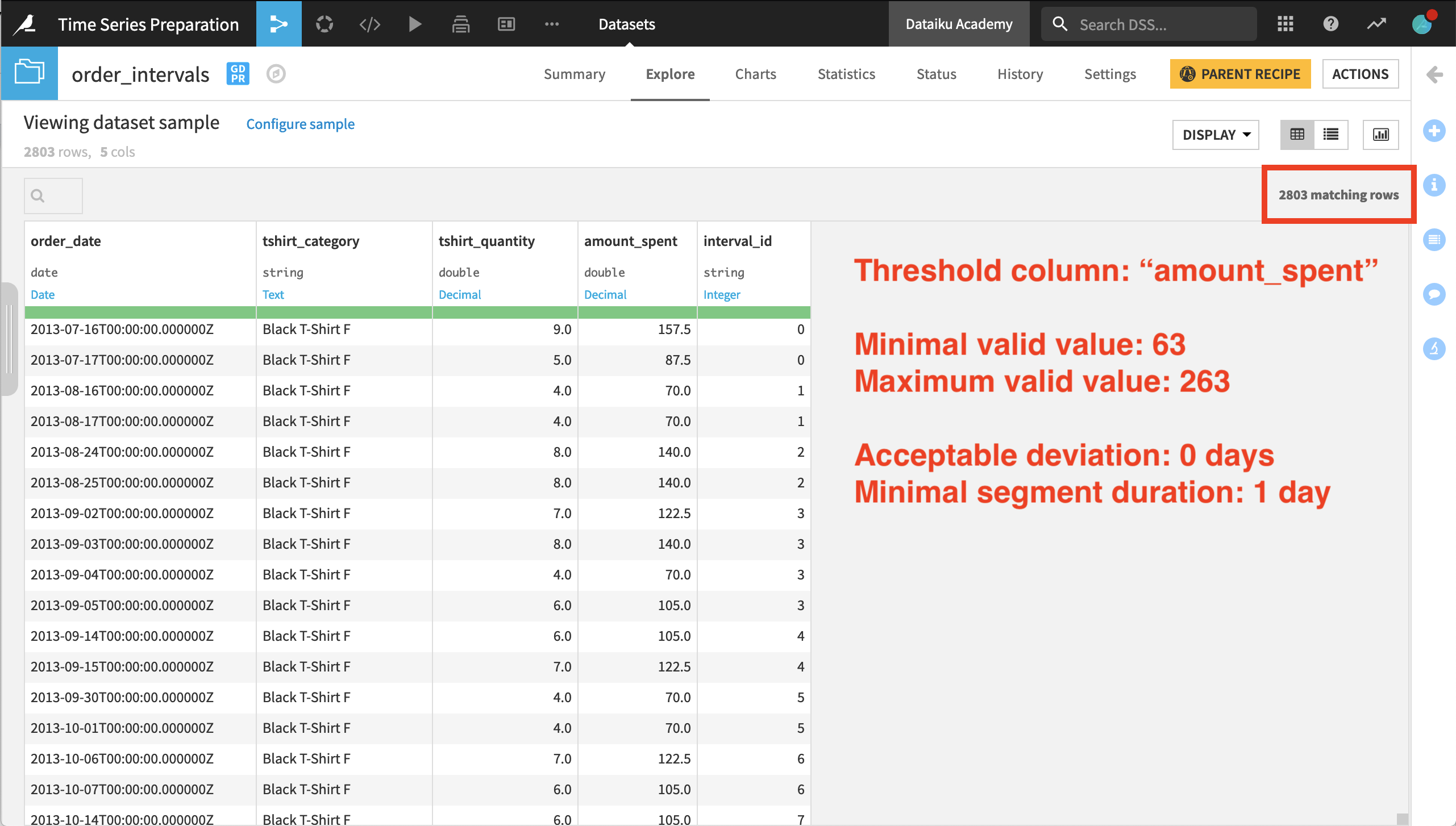
Let’s see how these results change as we adjust the segment parameters. Increasing this minimal segment duration parameter from 0 to 1 day imposes a stricter requirement for assigning an interval ID. After imposing this condition, the output includes about 70% of the rows returned when having both segment parameters at 0 days.

Now let’s also increase the flexibility of assigning interval IDs using the acceptable deviation parameter. We’ll increase the acceptable deviation from 0 to 1 day and observe the results.

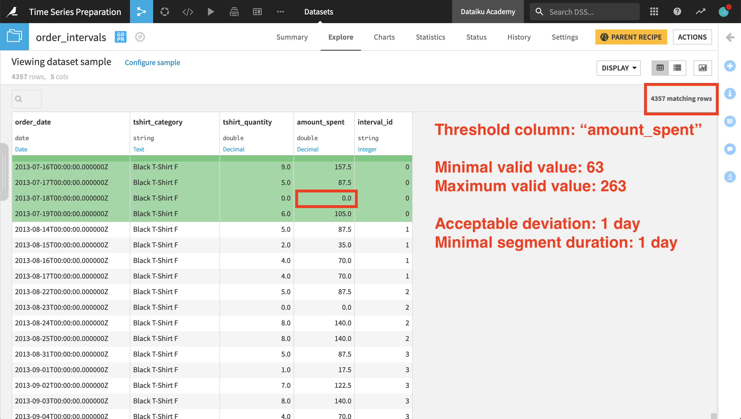
Shown in the image above, we still have fewer results than when both segment parameters were set at 0 days, but far more rows than the previous result where there was no acceptable deviation.

In the very first interval ID for the female Black T-shirt category, we can see the acceptable deviation parameter at work. The value of amount_spent for July 17th is in the range; the 18th is not, but then the value for the 19th is back in the range. Because the deviation lasts only one day, the value for the 18th is included in the interval.

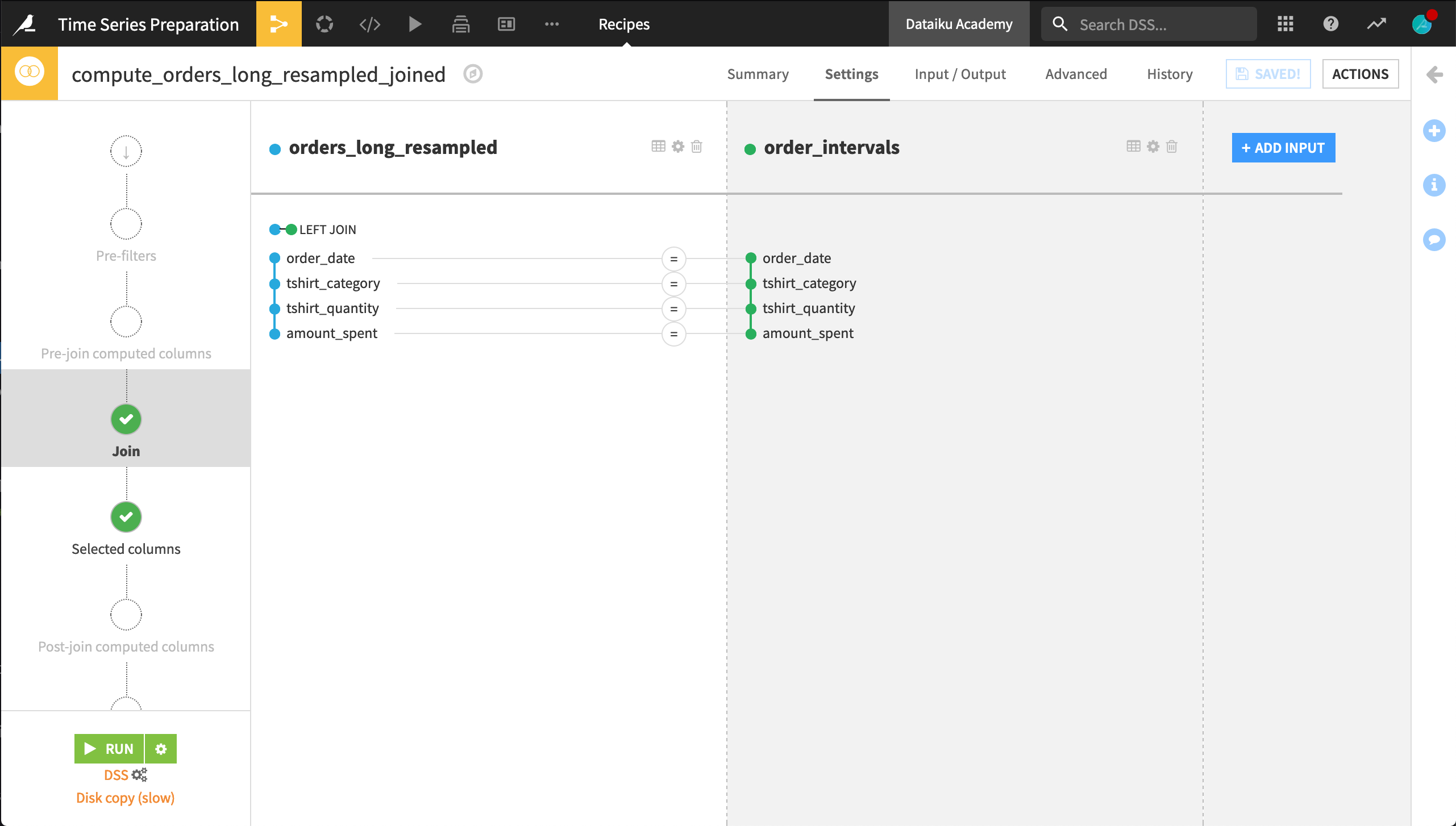
The Interval Extraction recipe returns rows from the input dataset that are assigned an interval ID. If we want to retrieve the rows that don’t receive an interval ID, we can do so by using a Join recipe.

Let’s explore the output of the Join recipe. The data is arranged first by chronological order instead of by product category. Using the Analyze tool on the interval_id column can show us the number of empty values.

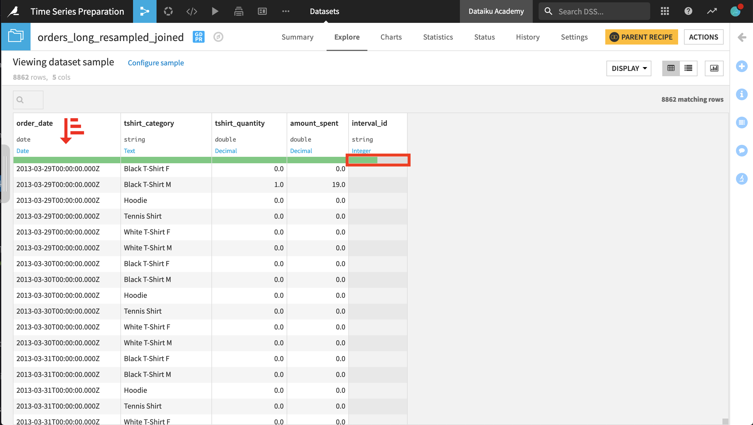
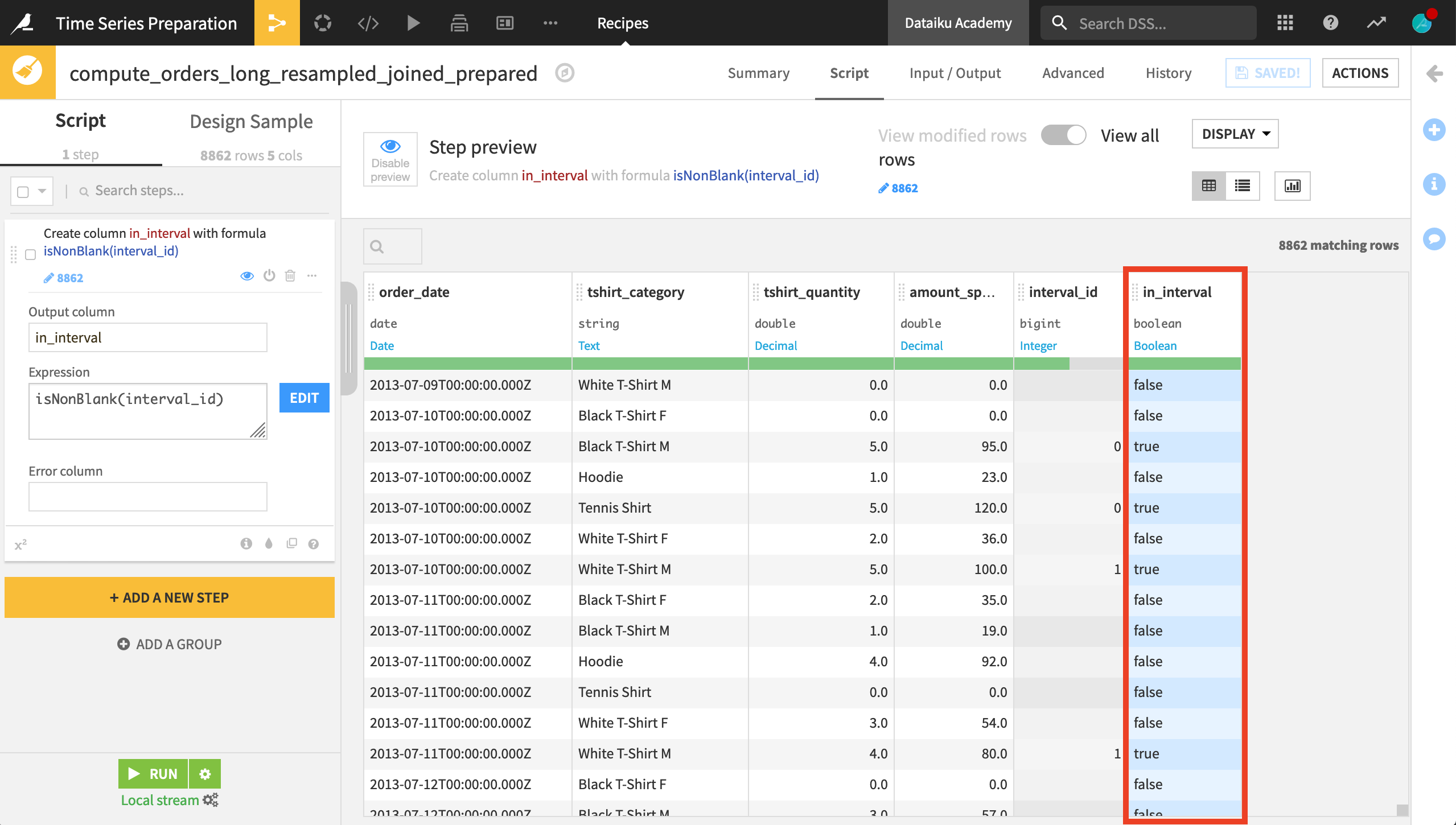
Once we have the dataset in this form, we can imagine building new features based on the interval_id column. For example, in a Prepare recipe, we could create a column classifying records that are within an interval or those that are not.

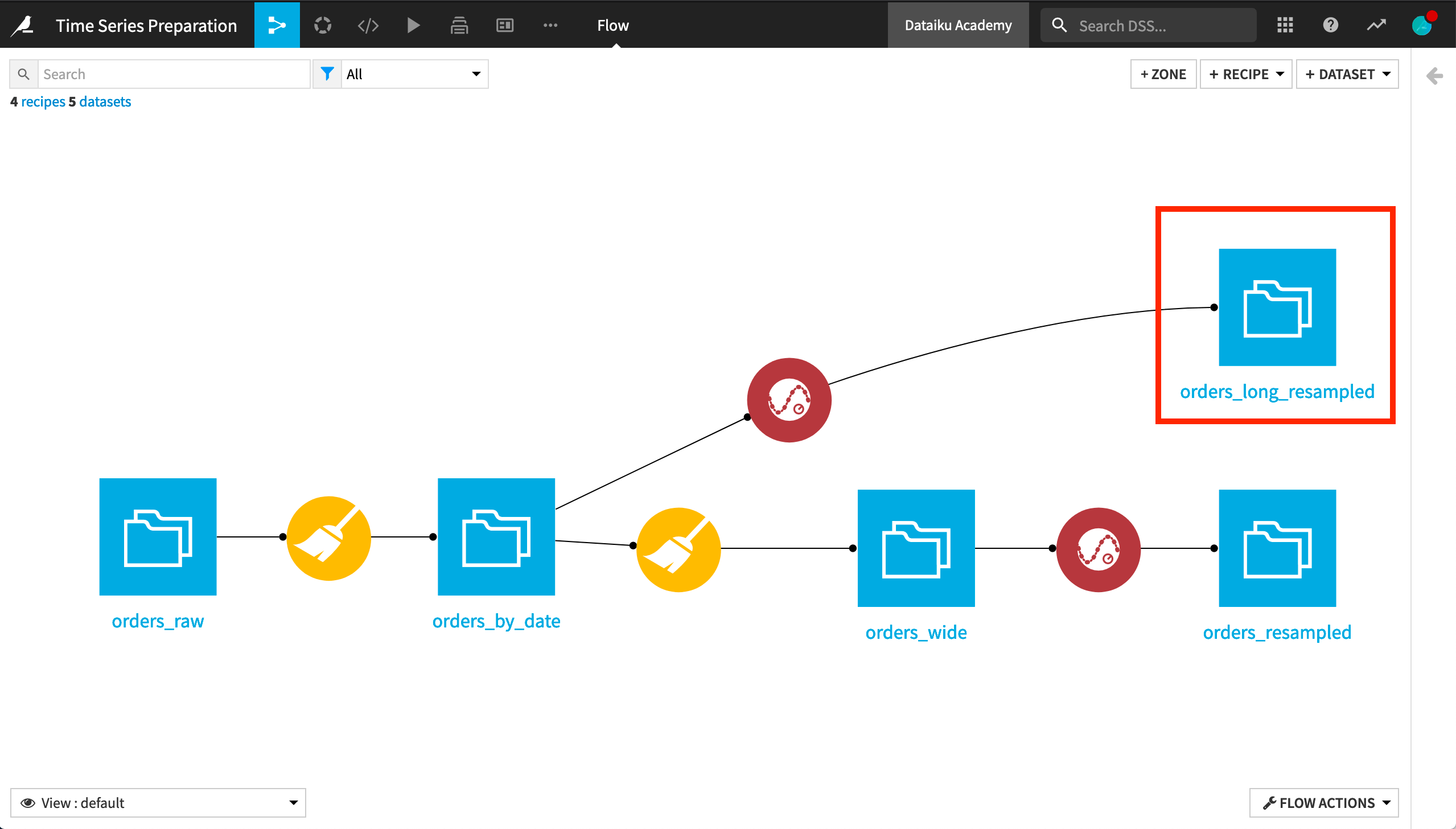
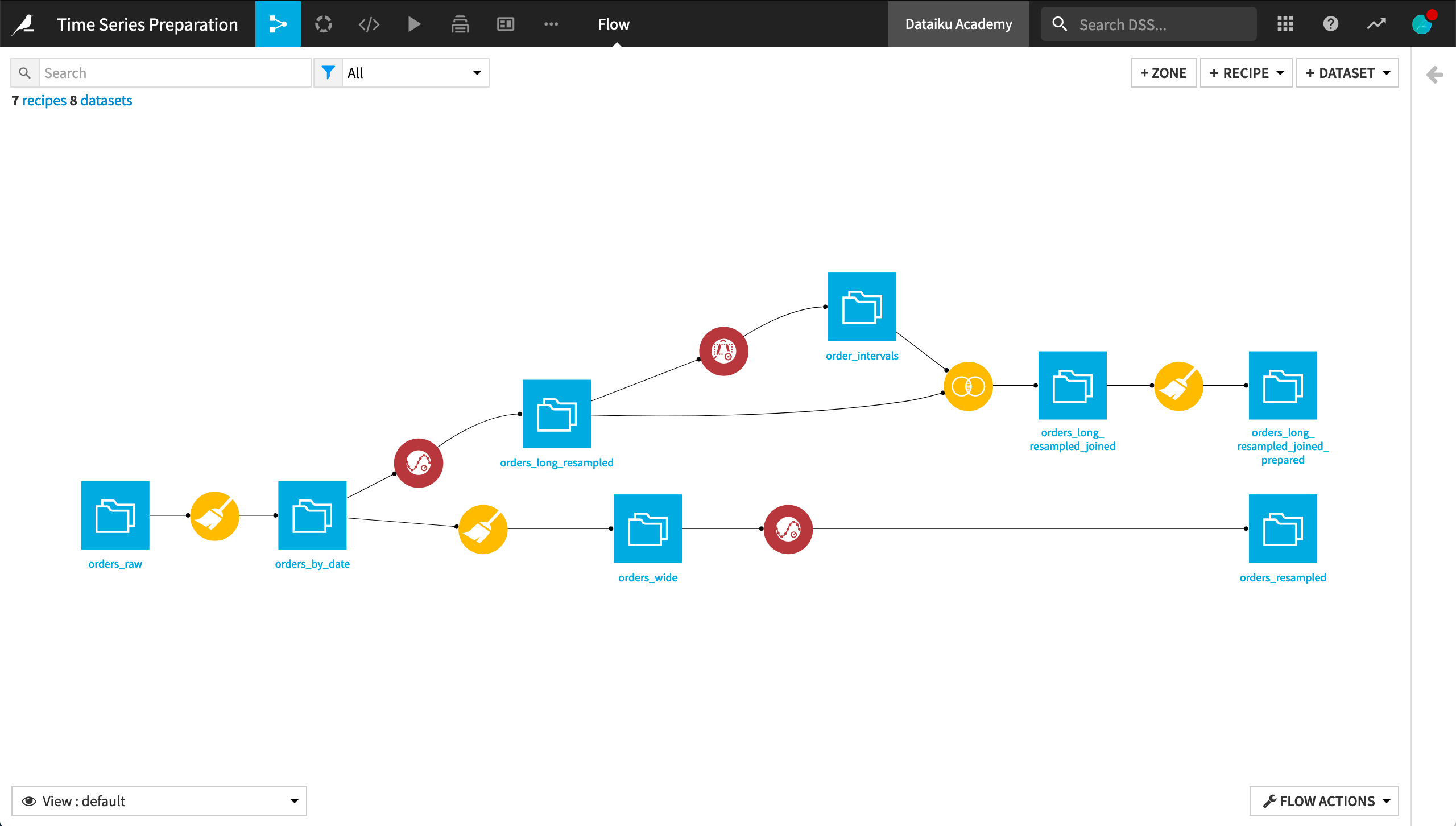
Once that step is complete, the final Flow should resemble the image below.

What’s next?

For many objectives, it’s also a good opportunity to use the time series Windowing recipe. This is the topic of the next section of this course on time series preparation.