Concept Summary: Time Series Windowing Pt 1

You are likely already familiar with the visual Window recipe in Dataiku DSS. It was introduced in the Visual Recipes Overview course.

In this lesson, we’ll draw on your knowledge of the visual Window recipe in order to present the Windowing recipe of the Time Series Preparation plugin, which is specifically geared to work with time series data.

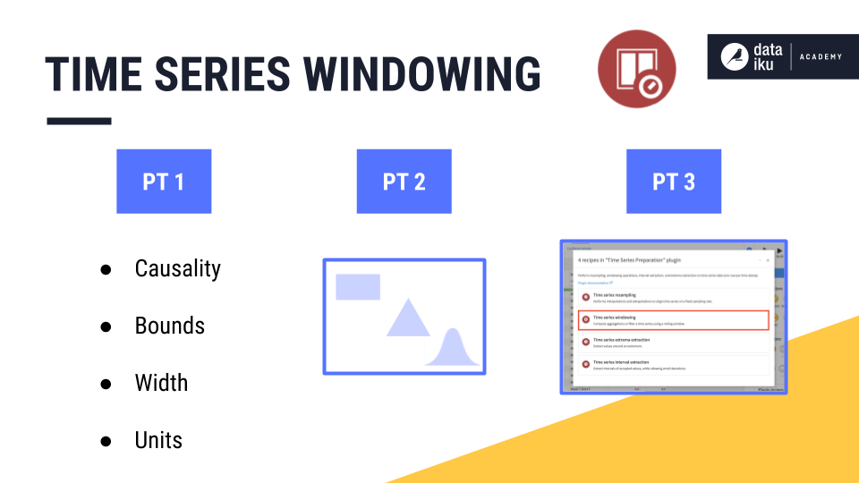
Using this recipe requires understanding a few different parameters, and so we have divided this lesson into 3 parts.

• In the first, we’ll dive into parameters like causality, bounds, width, and units.

• In the second part, we’ll introduce the concept of window shape.

• And in the last part, we’ll walk through a demo using the recipe.

Visual Window recipe

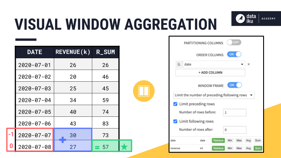
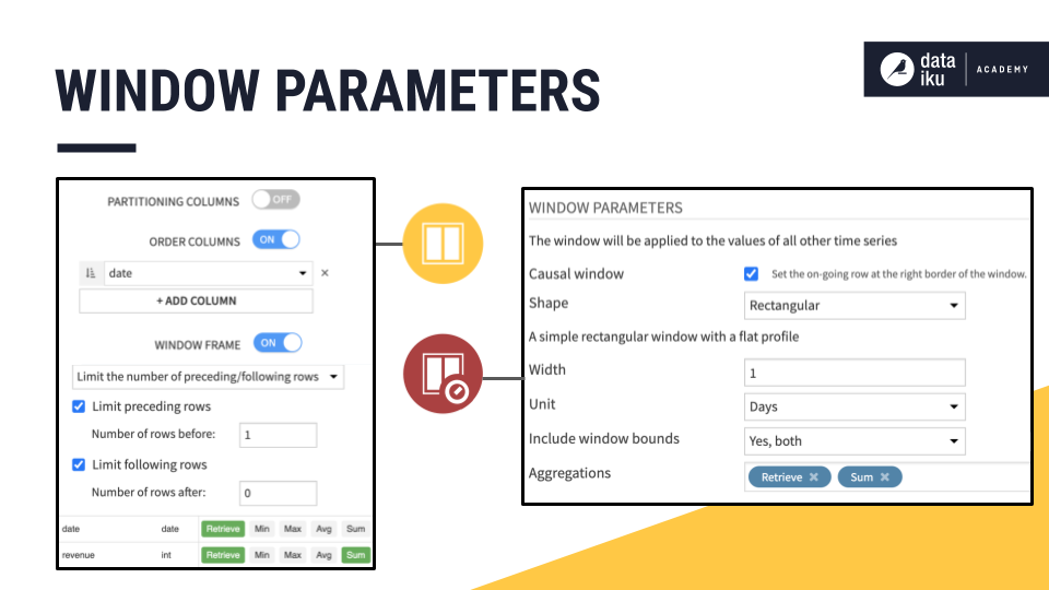
Let’s begin by reminding ourselves how to define window frames using the visual Window recipe.

• In the example below, we only have a single time series, and so we do not need to worry about partitioning columns.

• We can order rows by the “date” column in an increasing order.

• Then, we choose the rows to include in the window frame.

  • Here, let’s include 1 preceding row and 0 rows after the current row.

  • Once the window frame is set, we choose an aggregation, like a sum.

And then starting from the beginning, slide down, calculating the aggregation, row by row.

Time Series Windowing recipe

We can recreate this output with the time series Windowing recipe. You haven’t seen these parameters before, but they come directly from the dialog of the time series Windowing recipe.

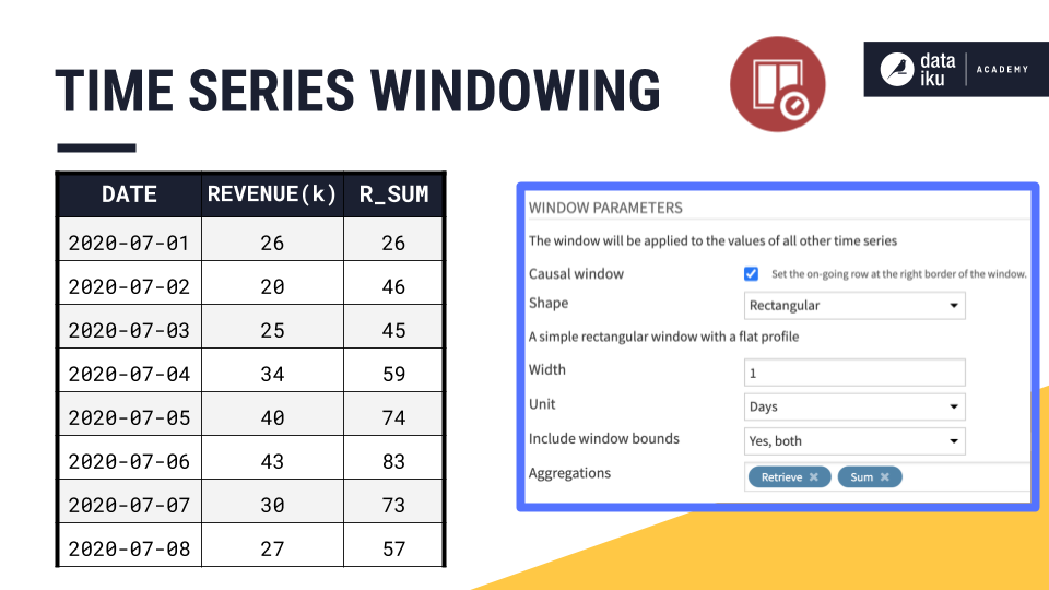
You’ll need to become familiar with terms like:

• Causality

• Shape

• Width

• Units

• Bounds

Causality

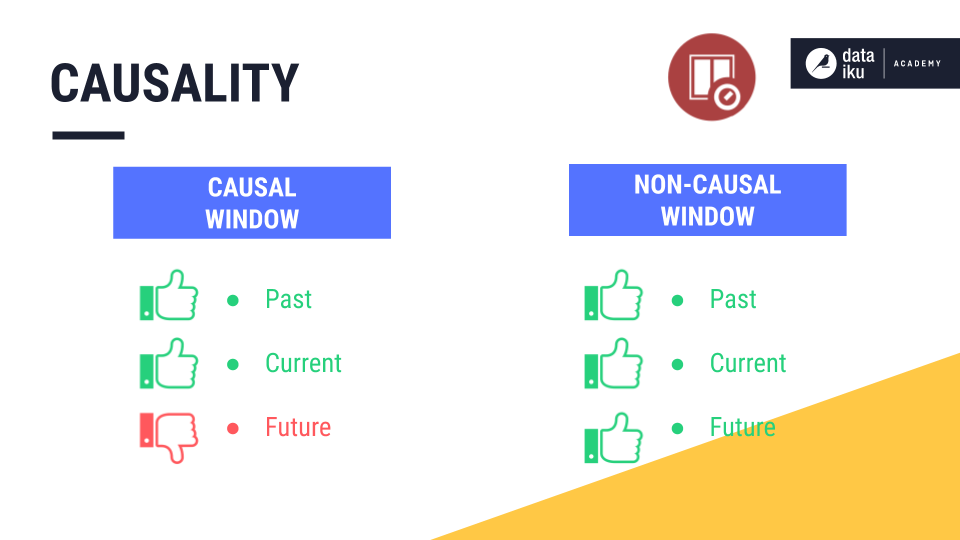
Let’s start with causality. In the time series windowing recipe, we first have to decide whether to build a causal or non-causal window:

• A causal window can only include past values and/or the current value in the window frame. It cannot include future values.

• A non-causal window (also known as a bilateral window), on the other hand, can include past, current, and future values.

The previous example using the visual Window recipe implemented a causal window frame because it included only past and current values.

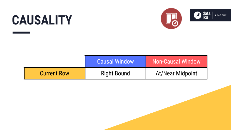
Causality is important because it defines the relationship between the current row and the window frame.

• In a causal window, the current row is always at the right bound of the window frame.

• But in a non-causal window, the current row is at or near the midpoint of the window frame, depending on whether the width is odd or even.

We’ll see how this works below.

Bounds

“Bound” is also a new term. You can think of it as the boundary or the edge of the window frame.

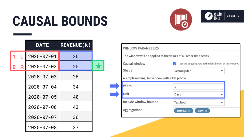
If July 2nd is our current row, in a causal window frame, that makes July 2nd the right bound. Knowing the right bound of a causal window is simple. It is always the current row.

The left bound is determined by two more parameters, width and units. We can think of the right bound as row zero and move back in time to set the left bound according to the width.

Since the width of this window frame is 1 day, if July 2nd is the right bound, then the left bound must be one day prior, July 1st.

It’s easier to see where the names for left and right bounds come from when looking at a line plot.

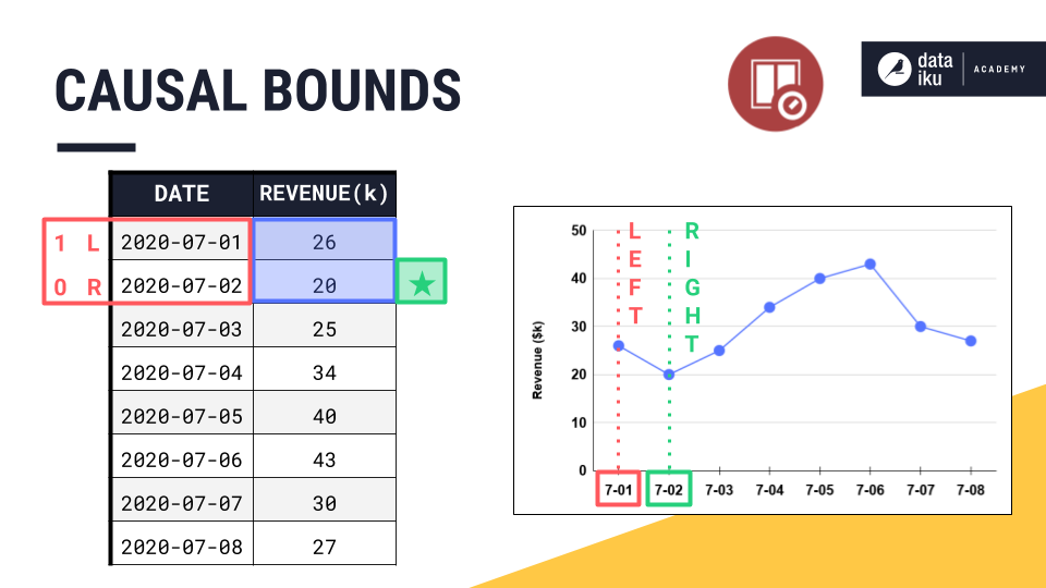
The right bound is the current timestamp, and the left bound is the earliest timestamp.

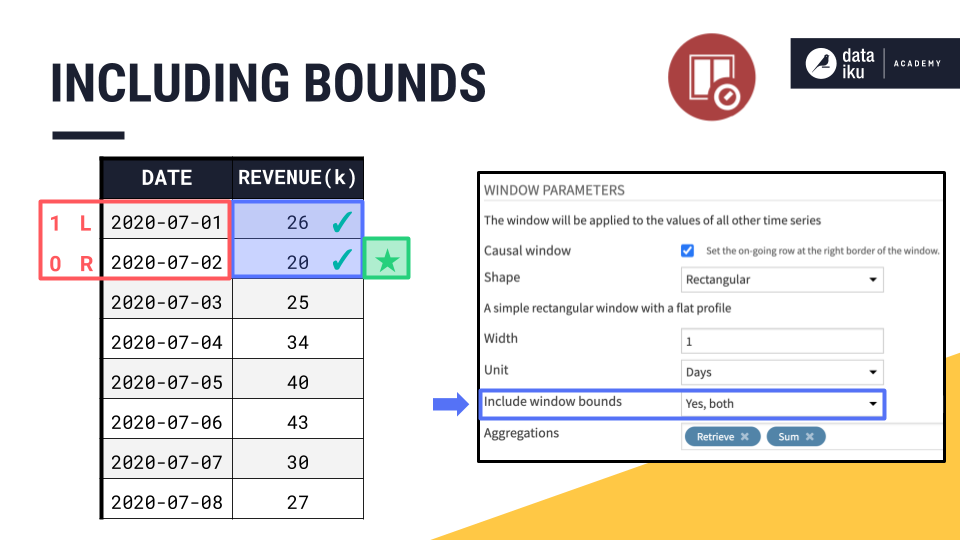
Once we have the placement of left and right bounds, we always have the option of whether to include or exclude them from the aggregation.

By default, the left bound is included in the aggregation, and the right bound, despite being part of the window frame, is excluded from any requested aggregations. This means, by default, the causal window frame in the Windowing recipe includes only past values.

In this example though, we are including both window bounds.

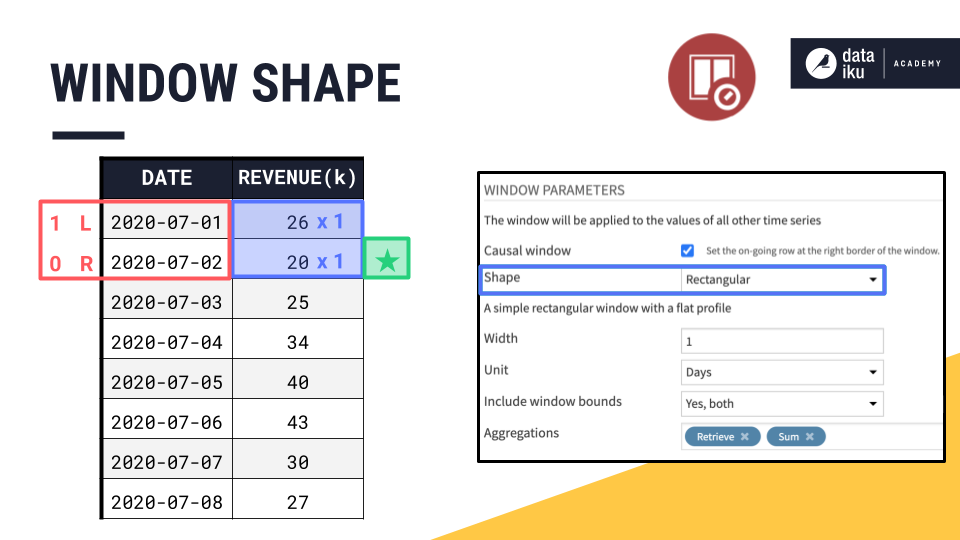
Window Shape

One remaining parameter needed to define a window frame is shape.

By selecting a rectangular window, all the values in the window are weighted equally, just as in the visual Window recipe. We’ll discuss the concept of window shape in more detail later in this summary.

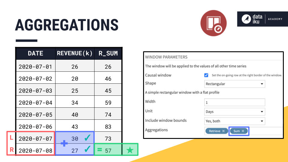
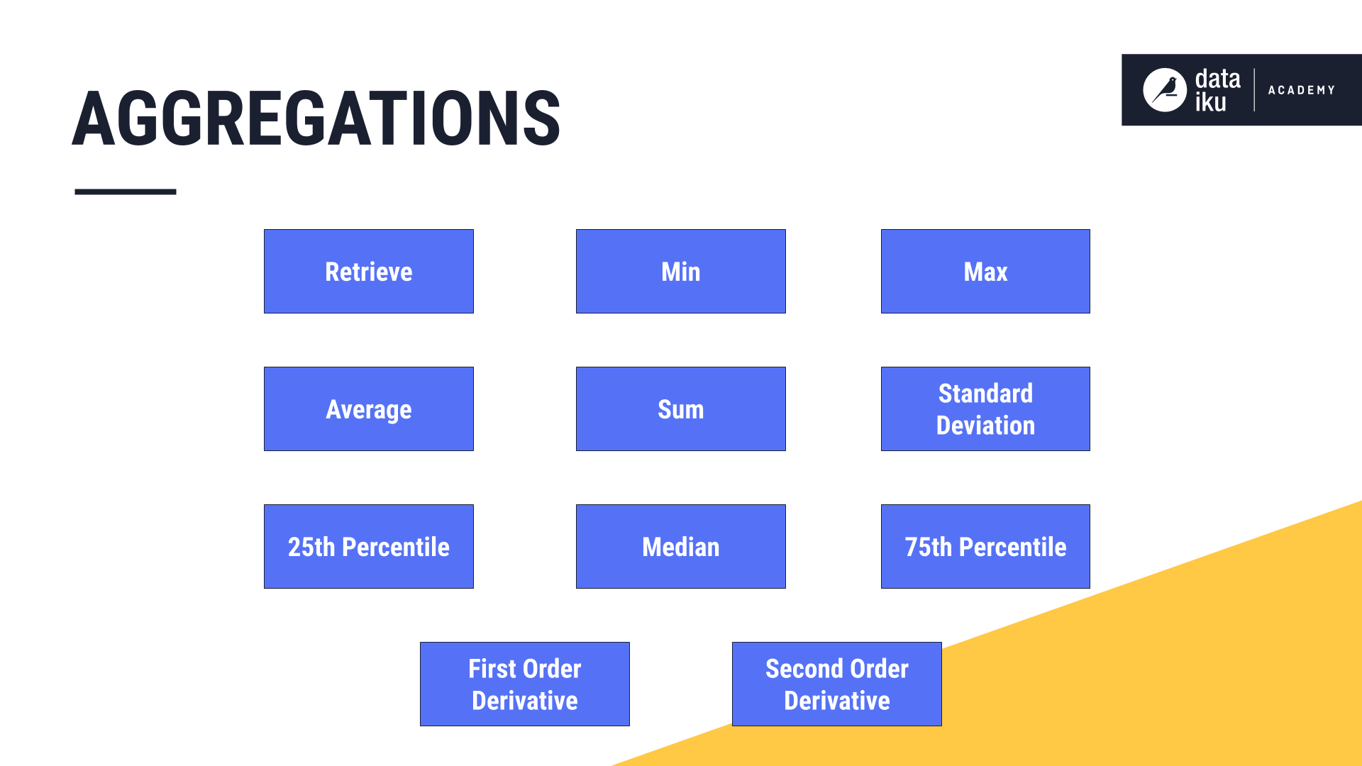
Window Aggregations

Now that we have a handle on causality, shape, width, units, and bounds, we can finally configure the aggregations.

“Retrieve” allows us to return the original column of values in the output, and “Sum” returns a column containing the sum of values in the window frame for each row.

We then slide down the dataset row by row, returning the requested aggregations, just like with the visual Window recipe.

Adjusting Time Series Windowing parameters

Now we have fully reproduced the example originally computed with the visual Window recipe, by using the time series Windowing recipe.

Let’s start adjusting some of these parameters to get a better feel for how they work.

Increasing Width

Let’s keep all of these parameters the same, but increase the width of the window frame from 1 to 2 days. What do we expect will happen?

Because this is a causal window, the right bound remains positioned at the current date. We only need to find the left bound.

• If the width is 2, we count 2 days instead of 1.

• If the width was 3, we count 3 days before the current day.

Notice how we said “3 days” instead of “3 rows”. In this example, previous days and previous rows are the same, but this will be an issue we address later when we have missing dates in the time series.

Changing Window Units

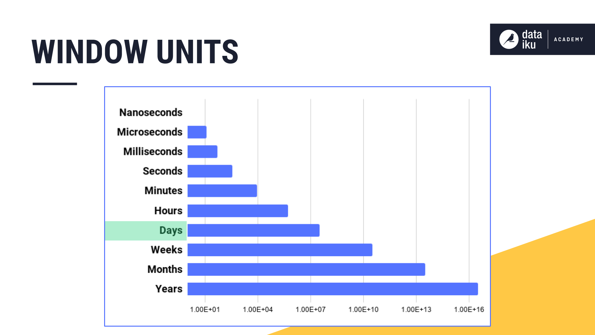
We are speaking in terms of days for this example, but depending on our data, this could be units as large as years or as small as nanoseconds.

Including/Excluding Bounds

Let’s finish the aggregation for this window frame. We have 4 values in a causal window frame of 3 days.

• If we are including both left and right bounds, then we sum all 4 values.

• Alternatively, we could include only the left bound.

• Or only the right bound.

• Or neither.

Changing Aggregations

And once we have the window frame defined, we can always change the aggregation. For example, we could change the aggregation from a rolling sum to a rolling average.

We could also choose from many other options, such as the median.

Non-Causal Windows

We can build a non-causal or bilateral window by un-checking this “Causal window” parameter.

Recall that, in a non-causal window, the current row is at or near the midpoint of the window frame instead of the right bound.

Once the causal box is unchecked, we no longer have the option to include or exclude the window bounds. Instead, we only have to think about the width.

If we start with a non-causal window and a width of 1 day, our average is just the current value. But as we increase the window width, what is happening becomes clear.

We are able to include values from both past and future timestamps in the window frame, centered around the current timestamp.

• When we have an odd width, like 3, it is easy to place the current row at the midpoint of the window frame.

• When we have an even width, like 4, the midpoint lies between two timestamps. We always choose the more recent one.

• At an odd width like 5, we’ll include two past values, the current value, and two future values.

Window Units

So far, we haven’t talked much about the units attached to the width of the window frame. But this is an important feature of the time series Windowing recipe not found in the visual Window recipe.

Imagine expanding a non-causal window from 5 to 7 days. This would give us a rolling weekly average in this case. We could achieve the same results by setting the width to 1 week instead of 7 days.

Imagine though, if we had a larger time series, where we wanted the width of the window to be a month or a year. On the orders dataset, we can see how adjusting the window frame units from days to weeks to months to years smooths out the trend on a line plot.

What’s next?

At this point, we have talked about causality, width, units, bounds, and aggregations. That leaves only shape.

We’ll introduce this topic in the Part 2 of this lesson on Time Series Windowing.