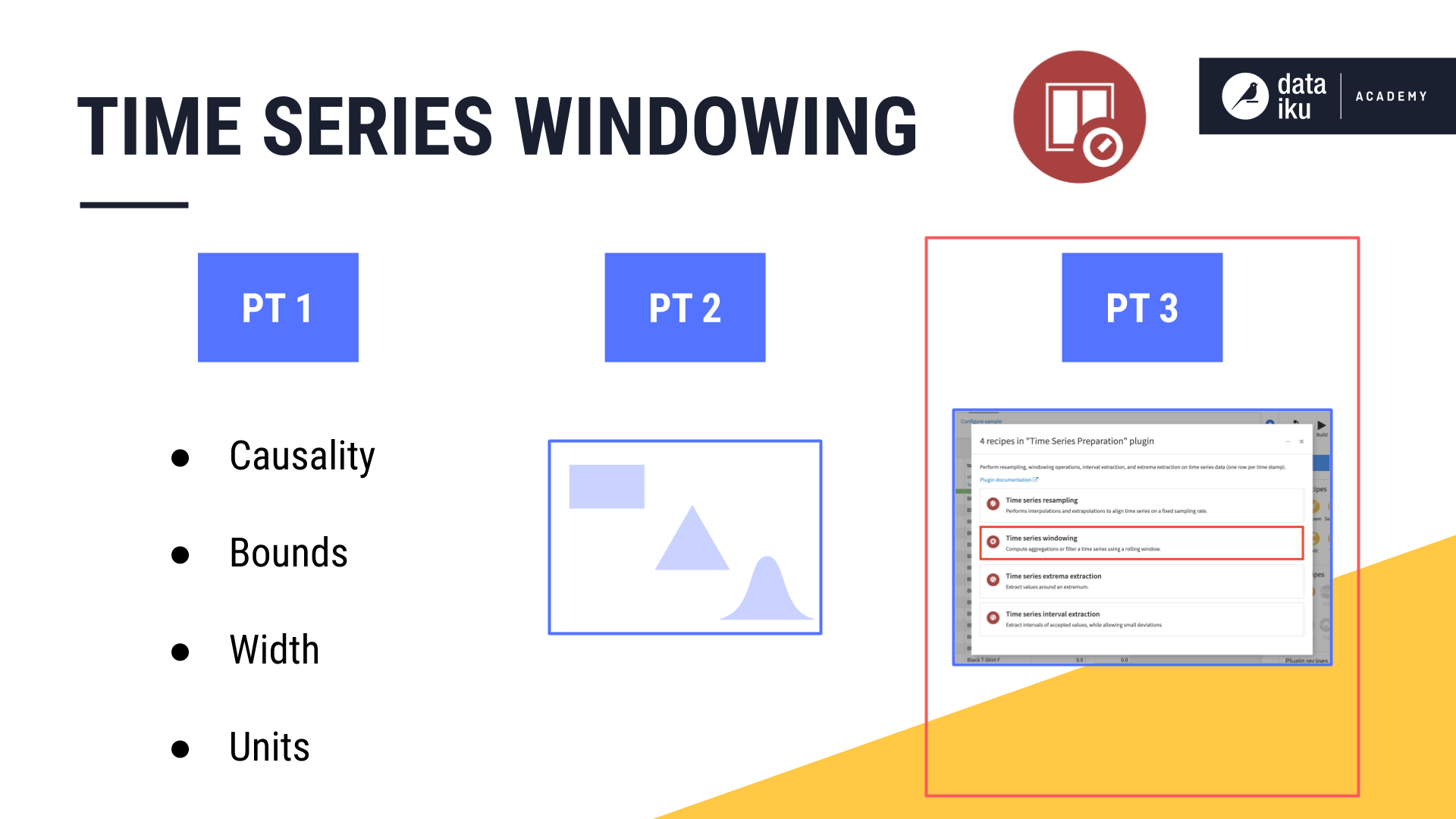
Concept Summary: Time Series Windowing Pt 3

After Parts 1 and 2 on the Time Series Windowing recipe, you know how parameters–like causality, shape, width, units, and bounds–all work together to define a window frame.

Now, actually doing so in Dataiku DSS should be easy. That’s what we’ll cover in Part 3.

Using the Time Series Windowing recipe

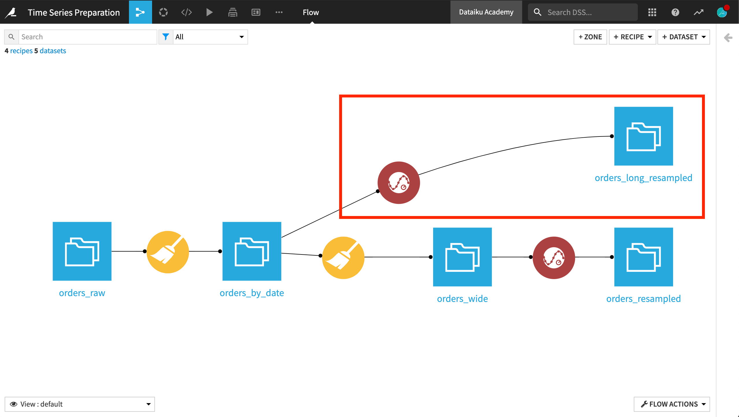
Let’s return to our familiar t-shirt orders data.

What do we need from our data in order to use the time series Windowing recipe?

• Like all other recipes in the plugin, we need a valid time series with a parsed date column.

• Unlike the Resampling recipe though, if we have multiple time series in the dataset, then the data must be stored in the long format.

The data does not necessarily need to be resampled in order to run the time series Windowing recipe, but you should be careful about failing to do so.

This is because, if timestamps are not equispaced, or if your data is missing some required interpolation or extrapolation steps, the output of the Windowing recipe may not represent what you expect.

For the input to the Windowing recipe, let’s use the resampled, long format time series, where we interpolated a constant value of 0 for dates with no sales. From this dataset, we are ready to build any kind of windows we need.

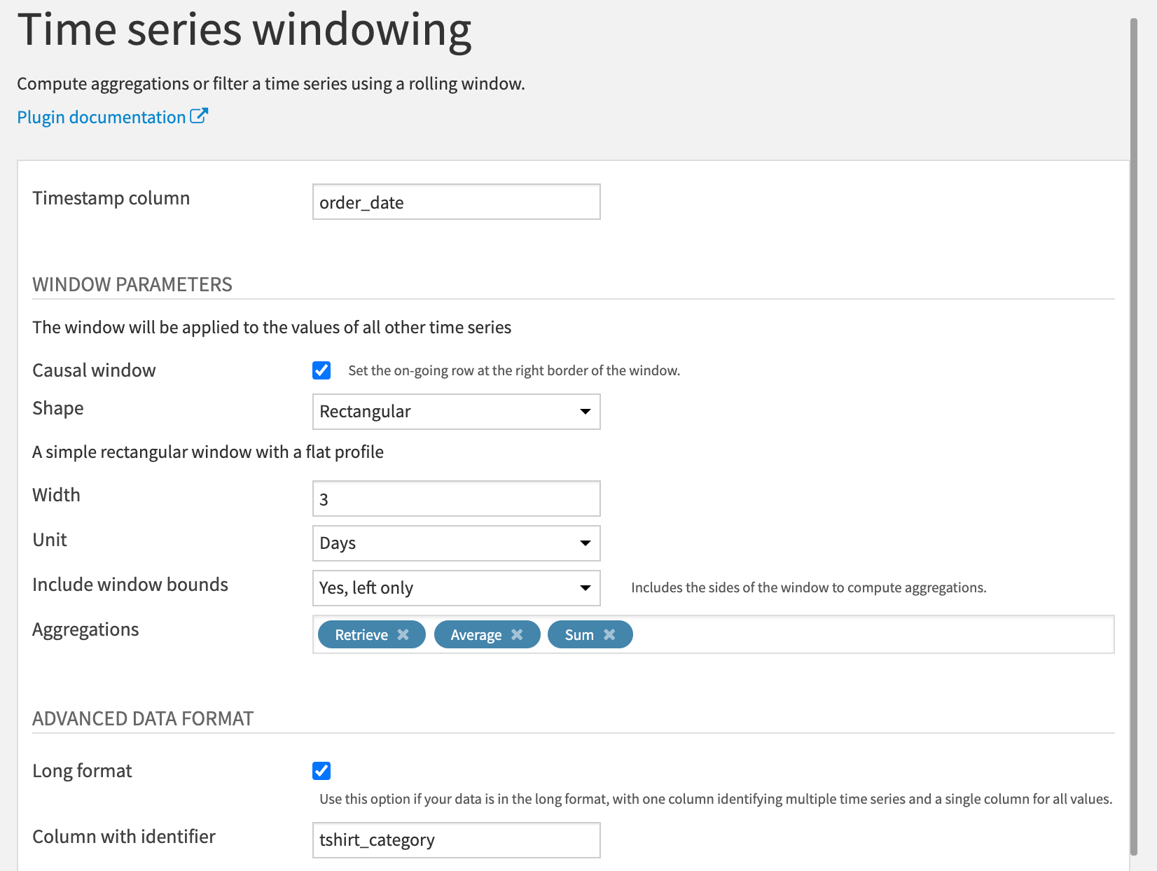
As with all recipes in the plugin, we first provide the name of the timestamp column.

We also know the data is in long format, with the “tshirt_category” column serving as the identifier column.

The Window parameters should look quite familiar by now.

You should experiment on your own by building different kinds of windows, but for now let’s build a causal, rectangular window of 3 days, including only the left bound.

We’ll retrieve our measurements, calculate the average, and find the sum using a rolling window.

In the output, observe that the numerical columns from the input dataset have been retrieved along with the timestamp and the identifier columns.

In addition, for each of the numerical columns, there are two new columns, one for each of the aggregates (average and sum).

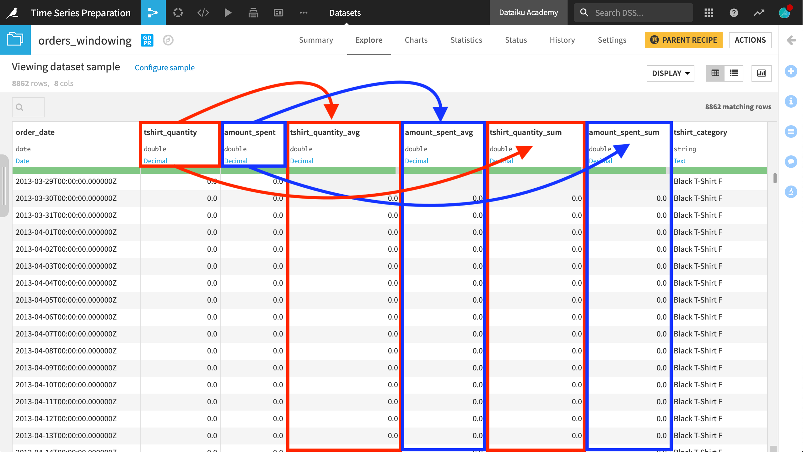
The results are sorted first by the identifier column groups, and then in ascending order by date.

Now it’s up to you to build your own windows that achieve your time series goals!

What’s next?

Congratulations! Once you have a handle on time series windowing, learn how the same knowledge of building window frames can be used in the Extrema Extraction recipe.