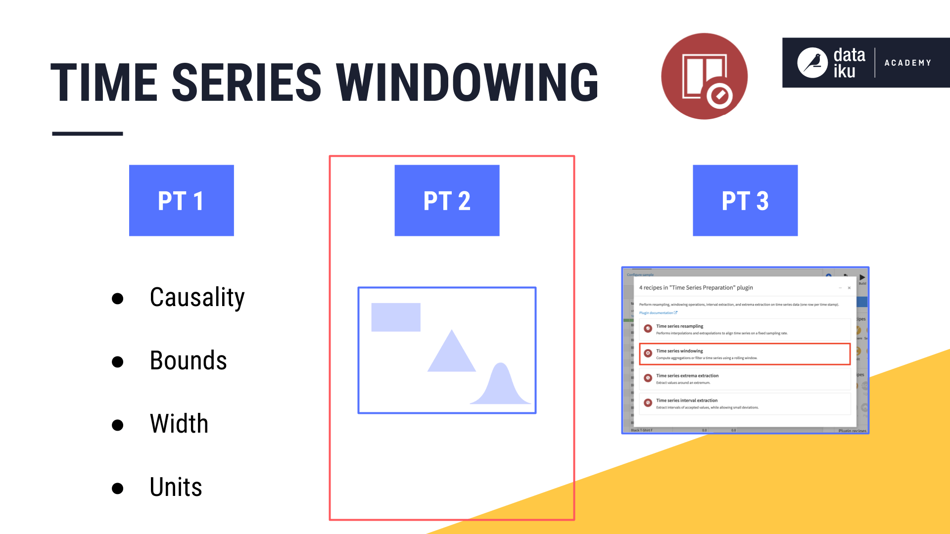
Concept Summary: Time Series Windowing Pt 2

In Part 1 of our lesson on the Time Series Windowing recipe from the Time Series Preparation Plugin, we talked about causality, width, units, bounds, and aggregations.

That leaves only shape, the topic of part 2. The shape of the window frame in all of the previous examples is a rectangle. What does this parameter mean?

Rectangular Window Frames

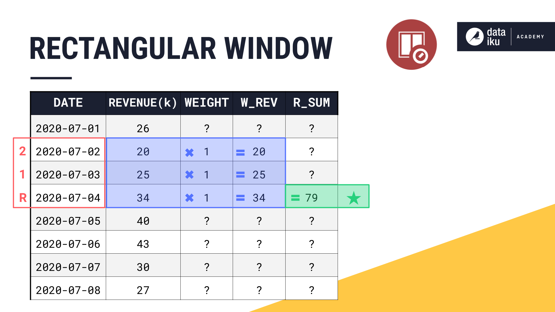
Consider a causal window of 2 days, including both left and right bounds in the aggregations. When calculating the rolling sum, it made no difference if a value was positioned at the beginning, middle, or end of the window frame.

In other words, we can think of all values in the rectangular window frame as having a weight of 1.

Two new columns in the table, weight and weighted revenue, will help us think through the shape parameter.

• DSS assigns a weight of 1 to all values contained in the rectangular window frame.

• If we multiply all of the original values by their weight of 1, we of course get the same output.

• We can then proceed with our aggregations in the same way as before, using the weighted revenue instead of the original revenue values.

Let’s take a graphical approach.

We can visualize a rectangular shape if we draw the horizontal width the same width as the window frame and assign a uniform vertical length of 1.

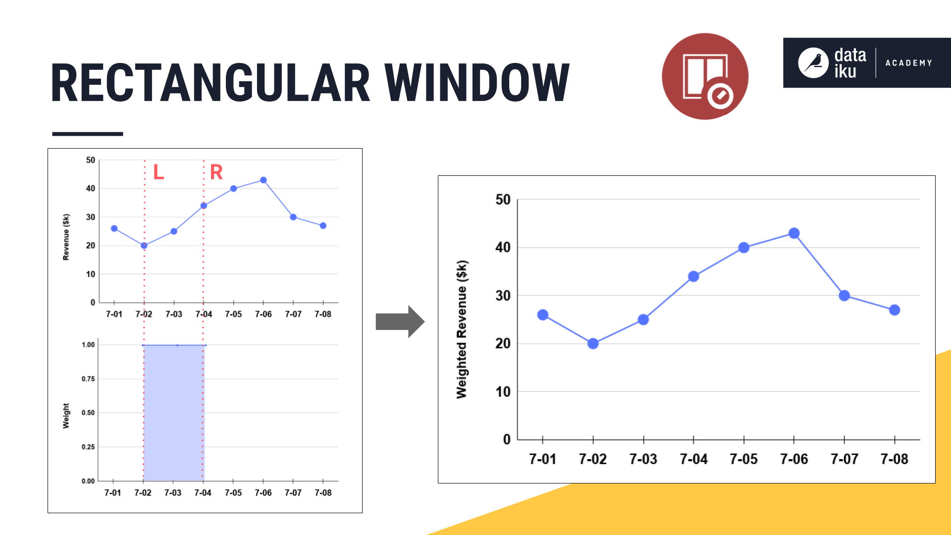
When we multiply each observation in the original line plot by its assigned weight, the weighted revenue is identical to the original revenue values.

Remember though that time series do not consist of independent observations. Perhaps we do not want to give equal weights to all values in the window frame. In some cases, we may want values in the center of the window frame to be of greater importance than those values on the edges.

Triangular Window Frames

We can imagine weighting the values in a window frame according to shapes other than a simple rectangle, such as a triangle, or a variety of other bell-shaped curves.

Let’s walk through this again with a new example. Below we have a non-causal window.

We will start with a width of 1 day and watch it expand into both past and future values, centered around the present. Instead of the usual rectangular window though, let’s make it a triangular window.

With a width of just 1 day, our results are the same as we’d find for a rectangular window. The weight can only be 1.

What happens to the weights as the width of the window frame expands? The general idea is to first find the center of the window frame. With an even width, the center falls between two rows. The center of the window frame will be the center of the triangle.

Think of the peak of the triangle as having a weight of 1. Then the weights decrease moving out towards the ends of the window frame. In a triangle window, that decrease is linear, making each row equally weighted at one-half.

Applying these weights, we get our weighted revenue. And from the weighted values, we can now calculate the aggregation as we normally would, in this case, a sum.

Let’s expand the width to 3 days, keeping all of the other parameters the same. First find the center. For a non-causal window of an odd width, that is the current timestamp. Assign the center of the window frame a weight of 1. Now decrease the weights linearly moving out from the center. Then just like before, sum the weighted values to get th e final result.

We can see this trend continue as we move to a width of 4 days. Finding the center. Assigning the weights based on the chosen shape. And using the weighted values to perform the requested aggregation.

For now, let’s stop at a width of 5 days and instead see what is happening on the line plot. As the width of the window frame increases, we can see how the weights assigned by the triangle change.

At the same time, we can plot the weighted revenue, the result of multiplying the original values by their assigned weight.

Shape as a Function

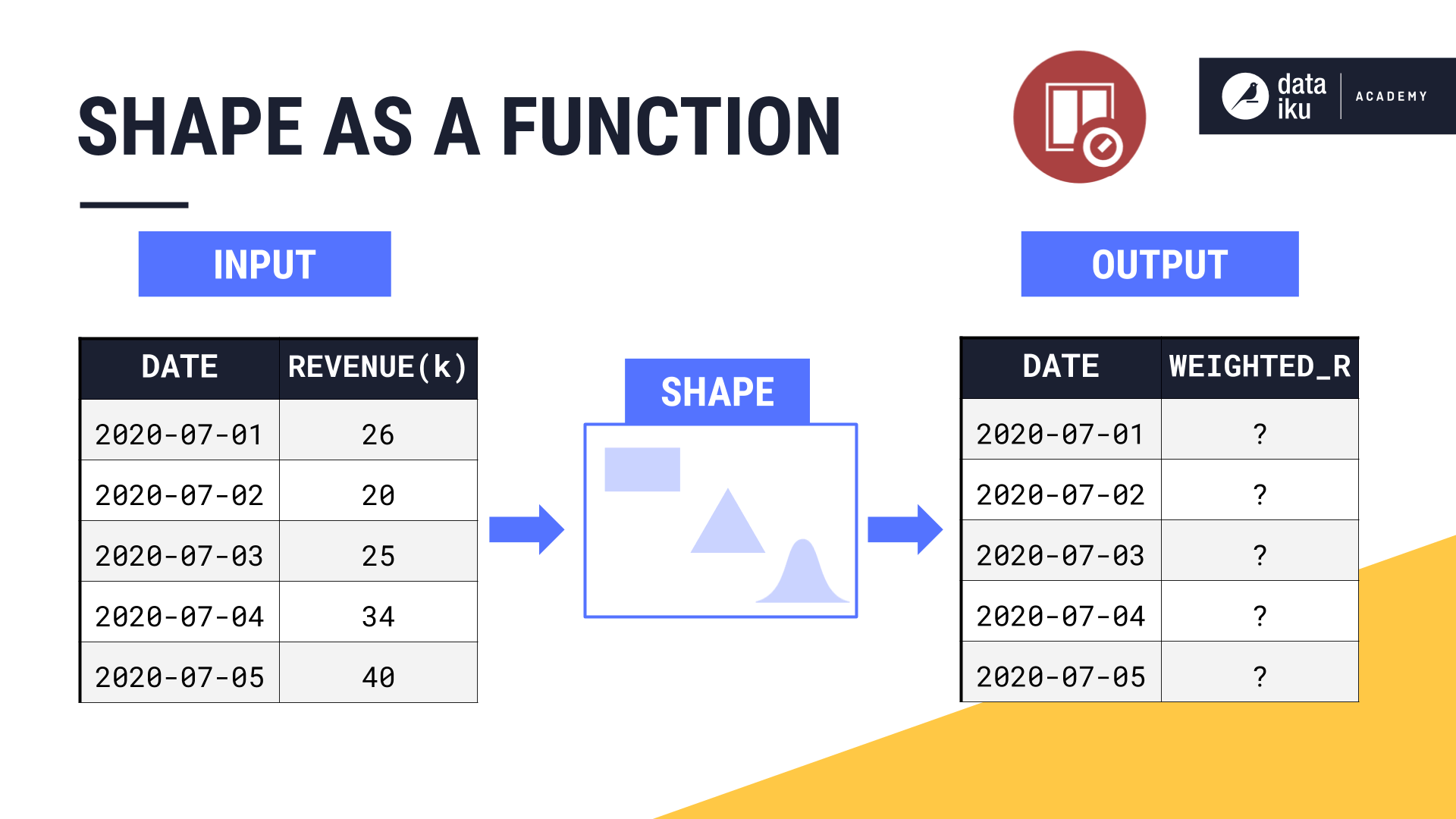
Having seen a few simple examples, you can begin to see that the shape parameter is just a function.

• The original values in your time series are the inputs to the shape function.

• The shape function assigns weights to these time series values based on the chosen shape and other window parameters like width and bounds.

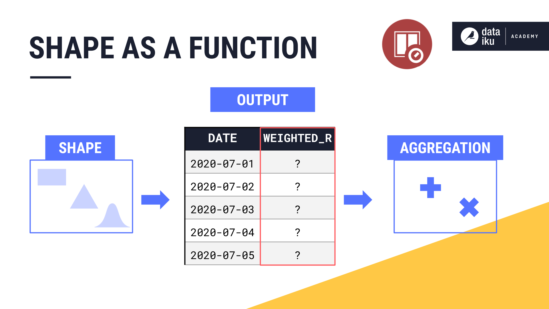
• After passing through the shape function, we have weighted values as output.

It’s these weighted values that will get passed to the aggregation step, like a rolling sum or an average.

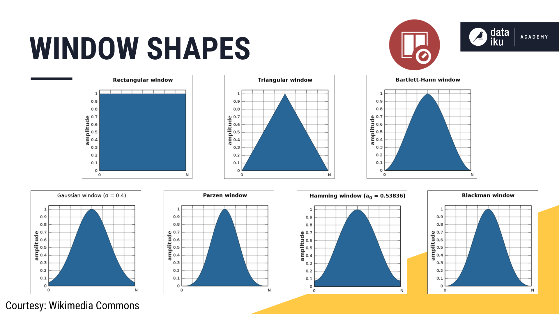
If the window shape is a rectangle, this function is very simple. All weights are just 1. If the shape is a triangle, the weights start at 1 in the center and decrease linearly.

But the shape function can be something more complex. The recipe makes it possible to assign weights according to a number of different bell-shaped curves.

What’s next?

Now that you know how parameters–like causality, shape, width, units, and bounds–all work together to define a window frame, actually doing so in Dataiku DSS should be easy.

And that’s exactly what we’ll cover in the part 3 of our lesson on the Time Series Windowing recipe.