Prepare the Trips Dataset
We now have data on bike stations and population counts, but what we are really interested in is the bike trips themselves. Let’s now explore the bike trips data.
In order to prepare the bike trips data so that it can be joined to station-level data, we will need to:
Download the raw trips data from the Capital Bikeshare website for years 2016 and 2017.
Prepare the trips data to extract the day of the week for each trip.
Pivot by customer type and day of the week to aggregate the individual trips. Doing so will allow you to compute the average trip duration by each customer type and day of the week.
Download the Raw Trips Data
First, let’s download the raw trips data in the same manner as the bike station data. Although we’ll work only with 2016 data first, download them both at this stage.
In the Flow, select + Recipe > Visual > Download.
Name the output folder
bike_dataand create the recipe.Add a new source with the following URL:
https://s3.amazonaws.com/capitalbikeshare-data/2016-capitalbikeshare-tripdata.zip.Add another source with the following URL:
https://s3.amazonaws.com/capitalbikeshare-data/2017-capitalbikeshare-tripdata.zip.Run the recipe to download both files.
Now read the 2016 data into Dataiku DSS.
Create a new Files in Folder dataset from the bike_data folder.
Within the Files tab, click on Show Advanced options and change the “Files selection” field from “All” to “Explicitly select files”.
Use the list files button on the right to display the contents of the folder.
Supply the name of the 2016 file (
1_2016-capitalbikeshare-tripdata.zip) to the “Files to include” field.Click Test to let Dataiku detect the CSV format and parse the data accordingly.
Rename the dataset
bike_dataand create it.
Note
Be mindful that the Gallery project is the “completed” version, and so has 2017 data loaded into the Flow.
Prepare the Trips Data
Just a few steps are needed to clean this data on bike trips.
In the Lab, create a new Visual Analysis on the bike_data dataset, accepting the default name, with the following steps in its script:
Parse in-place the Start date column into a proper date column in the format of
yyyy-MM-dd HH:mm:ss.Use the Extract date components processor on Start date to create one new column,
dow, representing the ‘Day of week’.
Note
Has Sunday been encoded as 1 or 7? You can find answers to questions like this by searching the help documentation in a number of ways. The Question icon at the top right provides one way to search in help. The full documentation can also always be found at doc.dataiku.com.
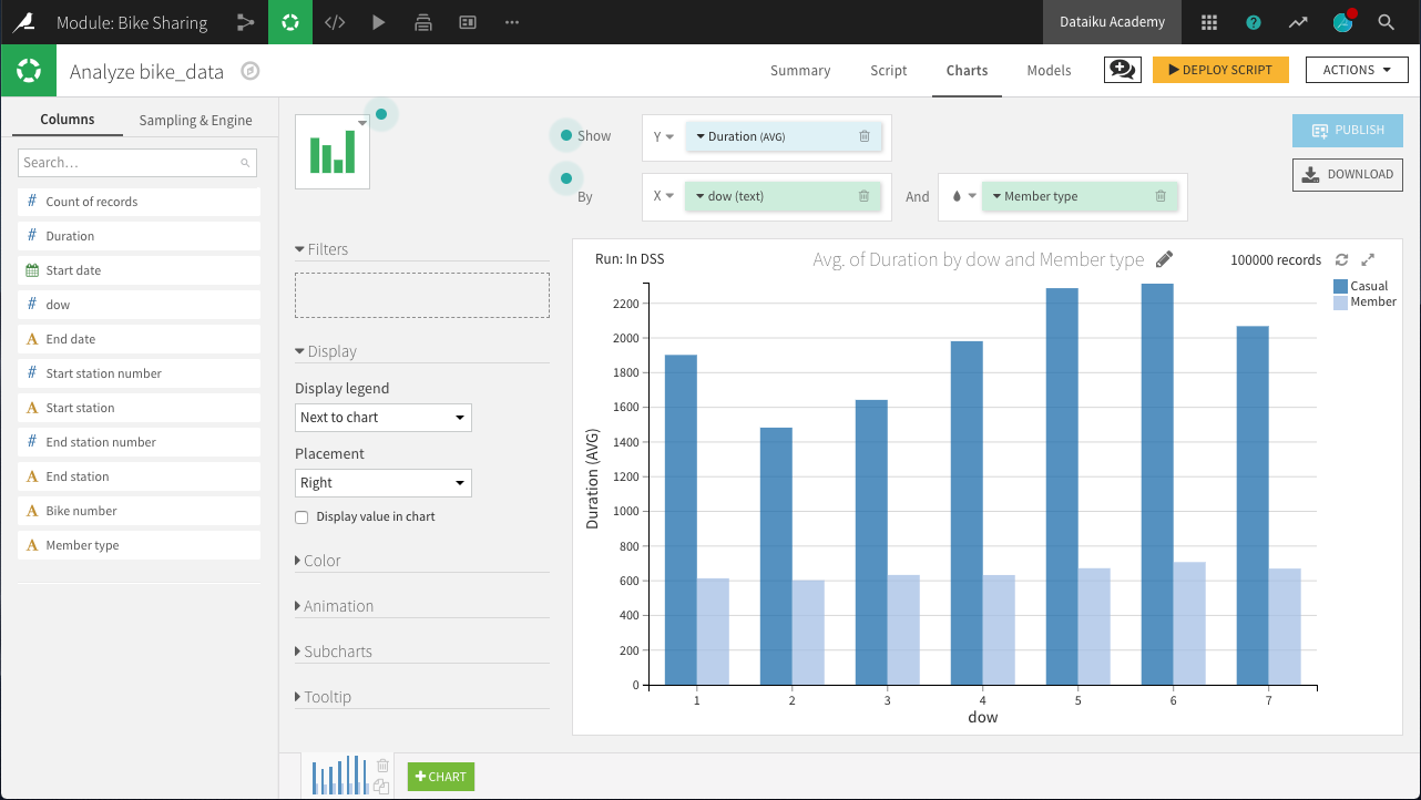
On the Charts tab, create a new histogram with:
Duration on the Y-axis
dow on the X-axis. Change the binning to “Treat as alphanum”.
Member type defining subgroups of bars.
Hint
Adjust the sample size to include enough data to populate the chart for each day of the week. For example, in the project shown in the screenshot below, the sample has been increased to the first 100,000 rows.

The chart above reveals a few interesting insights.
“Casual” customers tend to take trips that are significantly longer than “Member” users: approximately 40 minutes versus 12 minutes.
“Member” customers do not show much day-to-day variation in the duration of trips, while “Casual” customers make their longest trips on Friday, Saturday, and Sunday, and shortest trips on Tuesday and Wednesday: a difference of about 10 minutes.
Deploy the Visual Analysis script. Accept the default output name, bike_data_prepared. Build the new dataset now when deploying the script.
Now we have clean data on unique trips, but we need to aggregate it to the level of unique stations so that it can be merged with the station and block group demographic data. A Pivot recipe can help here!
Create pivoted features
In this step, we’ll create new features to support our analysis. More specifically, for each station, we want to compute the count of trips and average trip duration by member type and day of week.
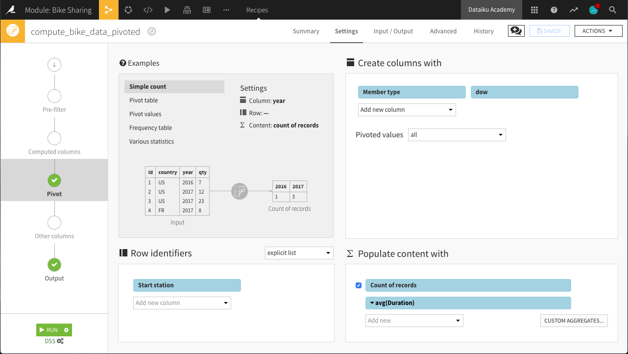
From the bike_data_prepared dataset, create a Pivot recipe.
Choose to pivot by Member type.
Name the output dataset
bike_data_pivoted.
In the Pivot step of the recipe:
Add dow as a second pivoting column (under “Create columns with”).
Choose to pivot all values instead of only the most frequent.
Select Start station as a row identifier.
Select Duration as a field to populate content with and choose Avg as the aggregation. Leave “Count of records” selected.

Run the recipe. The resulting dataset should have 29 columns:
1 for the Start station (the row identifier)
28 for the 7 days of the week x 2 member types x 2 statistics (count and average)
Here, we can interpret a column like Casual_1_Duration_avg as the average number of seconds of a bike trip by a Casual user on Day 1 (Monday).