Deep Learning for Time Series
As an alternative to traditional time series models like ARIMA, you can use deep learning for forecasting.
Objectives
This how-to walks through how to build a long short-term memory (LSTM) network, using Keras code in Dataiku’s Visual Machine Learning.
Prerequisites
You should have some experience with Deep Learning with code in Dataiku.
You should have some familiarity with Keras.
You will need access to a code environment with the necessary libraries. When creating a code environment, you can add sets of packages on the Packages to Install tab. Choose the Visual Deep Learning package set that corresponds to the hardware you’re running on.
Preparing the Data
We’ll work with a dataset containing the daily minimum temperatures recorded in Australia over the course of a decade (1981-1990). Download the data in CSV format, then create a new project and upload the CSV to a new dataset.
Parse Dates
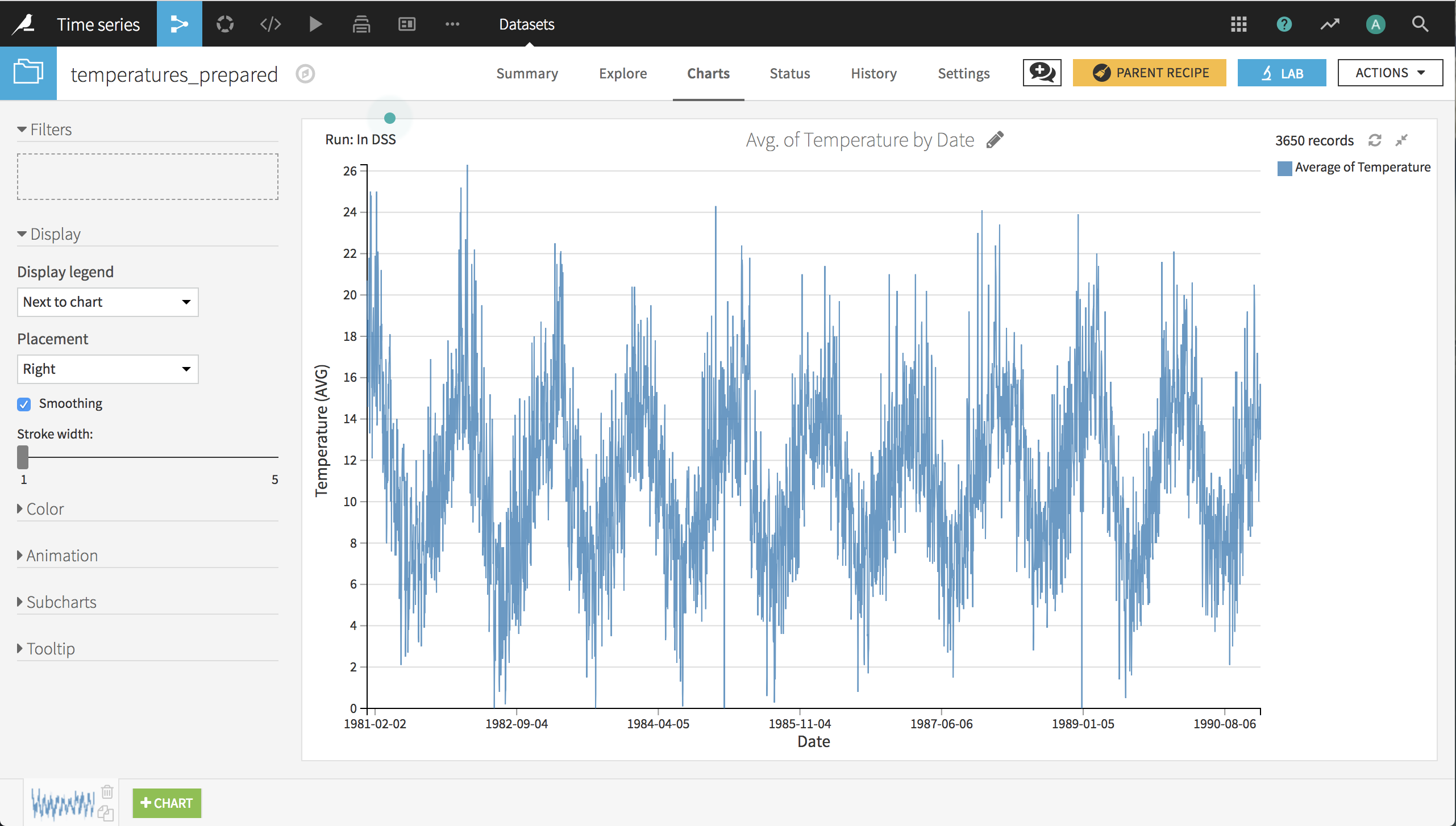
The first step in preparing the data is simply to parse the dates from string format into date format, using a Prepare recipe. In the prepared dataset, you can create a basic line chart of the temperature by date, which reveals that the data is quite noisy. Therefore our model will probably only learn the general trends.

Create Windows
The next step is to create windows of input values. We are going to feed the LSTM with windows of 30 temperature values, and expect it to predict the 31st. We do this with a Python code recipe that serializes the window values in string format. The resulting dataset has 3 columns: the date of the target measurement, a vector of 30 values of “input” measured temperatures, and the target temperature.
import dataiku
import pandas as pd, numpy as np
from dataiku import pandasutils as pdu

# Read recipe inputs
generated_series = dataiku.Dataset("temperatures_prepared")
df_data = generated_series.get_dataframe()

steps = []
x = []
y = []

## Set the number of historical data points to use to predict future records
window_size = 30

## Create windows of input values
for i in range(len(df_data) - window_size - 1):
    subdf = df_data.iloc[i:i + window_size + 1]
    values = subdf['Temperature'].values.tolist()
    step = subdf['Date'].values.tolist()[-1]

    x.append(str(values[:-1]))
    steps.append(step)
    y.append(values[-1])

df_win = pd.DataFrame.from_dict({'date': steps, 'inputs': x, 'target': y})


# Write recipe outputs
series_window = dataiku.Dataset("temperature_window")
series_window.write_with_schema(df_win)
Split the Data
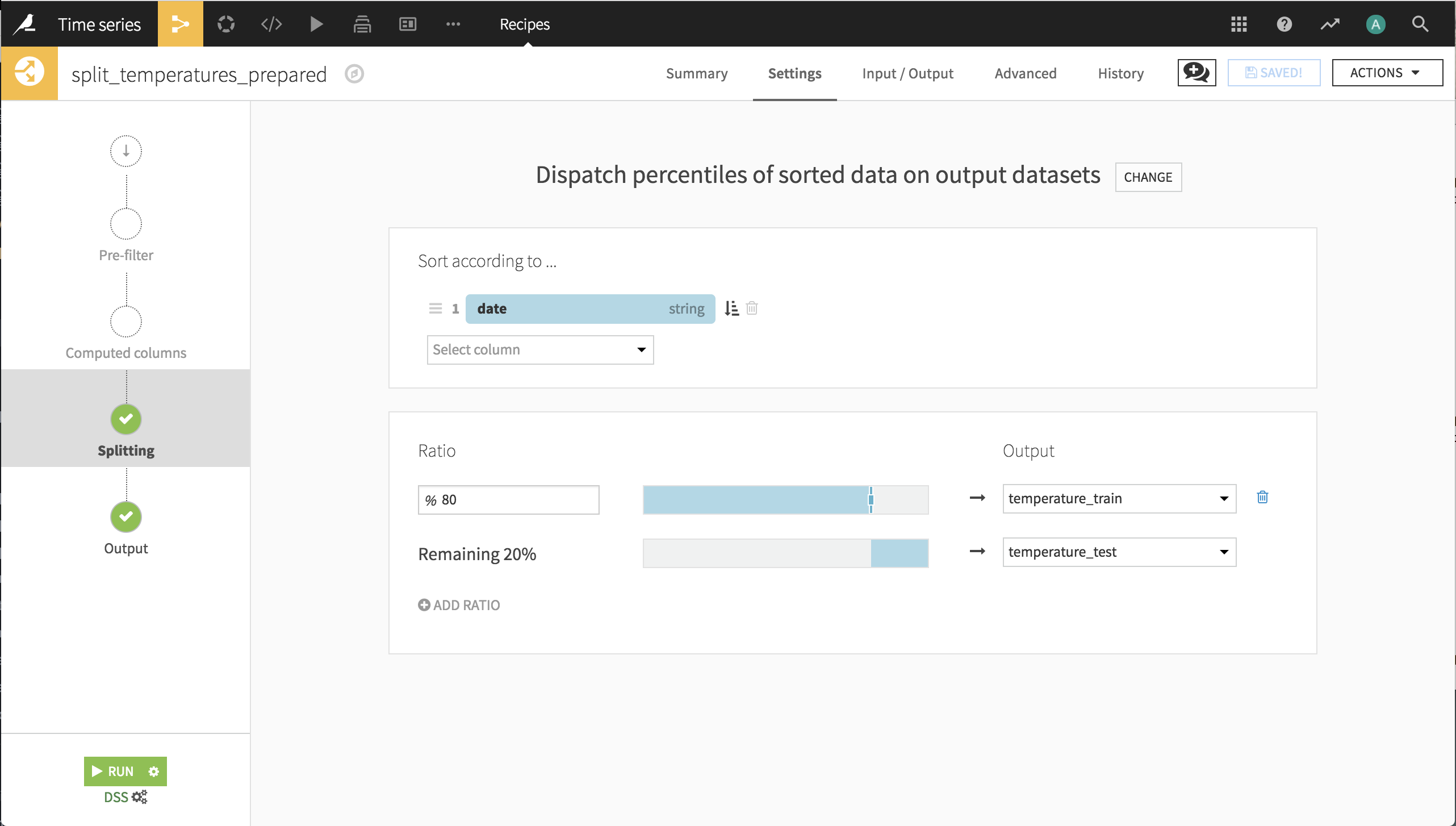
Finally we are ready to divide the dataset into train and test sets. The model is trained on the first 8 years of data, then tested on the final 2 years of data.

The Deep Learning Model
In a Visual Analysis for the training dataset, create a new model with:
Prediction as the task,
target as the target variable
Expert mode as the prediction style
Deep learning as the Expert mode, then click Create
This creates a new machine learning task and opens the Design tab for the task. On the Target panel, verify that Dataiku DSS has correctly identified this as a Regression type of ML task.
Features Handling with a Custom Processor
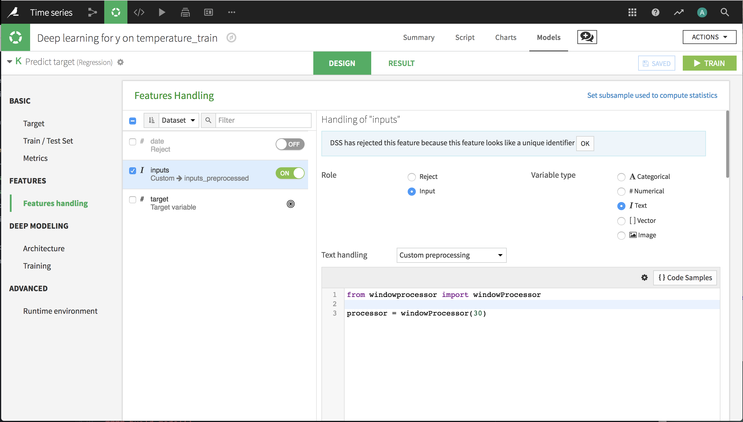
On the Features Handling panel, verify that date has been rejected as an input. inputs should, by default, also be rejected as an input because its values appear to be unique. We need a custom processor that unserializes the input string to a vector, and then normalizes the temperature values to be between 0 and 1.
To create the custom processor, from the top navigation bar go to the Code menu > Libraries. Create a new file called windowprocessor.py. The contents of the file should be as follows. It implements the following methods:
fit(), which computes the maximum and minimum values of the datasettransform(), which normalizes the values to be between 0 and 1_convert(), which transforms the data from an array of strings to a 2-dimensional array of floats
import numpy as np

class windowProcessor:
    def __init__(self, window_size):
        self.window_size = window_size

    def _convert(self, x):
        m = np.empty((len(x), self.window_size))
        for i in range(len(x)):
            c = np.array(eval(x[i]))

            m[i, :] = np.array(eval(x[i]))
        return m

    def fit(self, x):
        m = self._convert(x)
        self.min_value, self.max_value = m.min(), m.max()

    def transform(self, x):
        m = self._convert(x)
        return (m - self.min_value) / (self.max_value - self.min_value)
Back in the Features Handling panel of the deep learning model, turn on inputs as a feature. Select Text as the variable type. Select Custom preprocessing as the type of text handling. Erase the default code and input the following. This calls the custom processor and tells it that our window has 30 values.
from windowprocessor import windowProcessor

processor = windowProcessor(30)
This custom features handling creates a new input to the deep learning model called inputs_preprocessed. We’ll use that in the specification of the deep learning architecture.

Deep Learning Architecture
We need to import the LSTM and Reshape layers in order to specify our architecture. Replace the first line of code with the following.
from keras.layers import Input, Dense, LSTM, Reshape
We now have to create our network architecture in the build_model() function. Delete the default contents of build_model() and insert the following.
# This input will receive all the preprocessed features
window_size = 30

input_main = Input(shape=(window_size,), name="inputs_preprocessed")

x = Reshape((window_size, 1))(input_main)
x = LSTM(100, return_sequences=True)(x)
x = LSTM(100, return_sequences=False)(x)

predictions = Dense(1)(x)

# The 'inputs' parameter of your model must contain the
# full list of inputs used in the architecture
model = Model(inputs=[input_main], outputs=predictions)

return model
There are three hidden layers. First is a Reshape layer, to convert from a shape of (batch_size, window_size) to (batch_size, window_size, dimension). Since we only have one input variable at each time step, the dimension is 1. After the reshaping, we can stack 2 layers of LSTM. The output layer is a fully connected layer, Dense, with one output neuron. By default its activation function is linear, which is appropriate for a regression problem.
We’ll make no changes to the compile_model() function or the Training panel. If you have multiple code environments for deep learning, on the Runtime Environment panel, you should confirm that Dataiku has selected the code environment you want to use with this ML task.
Model Results
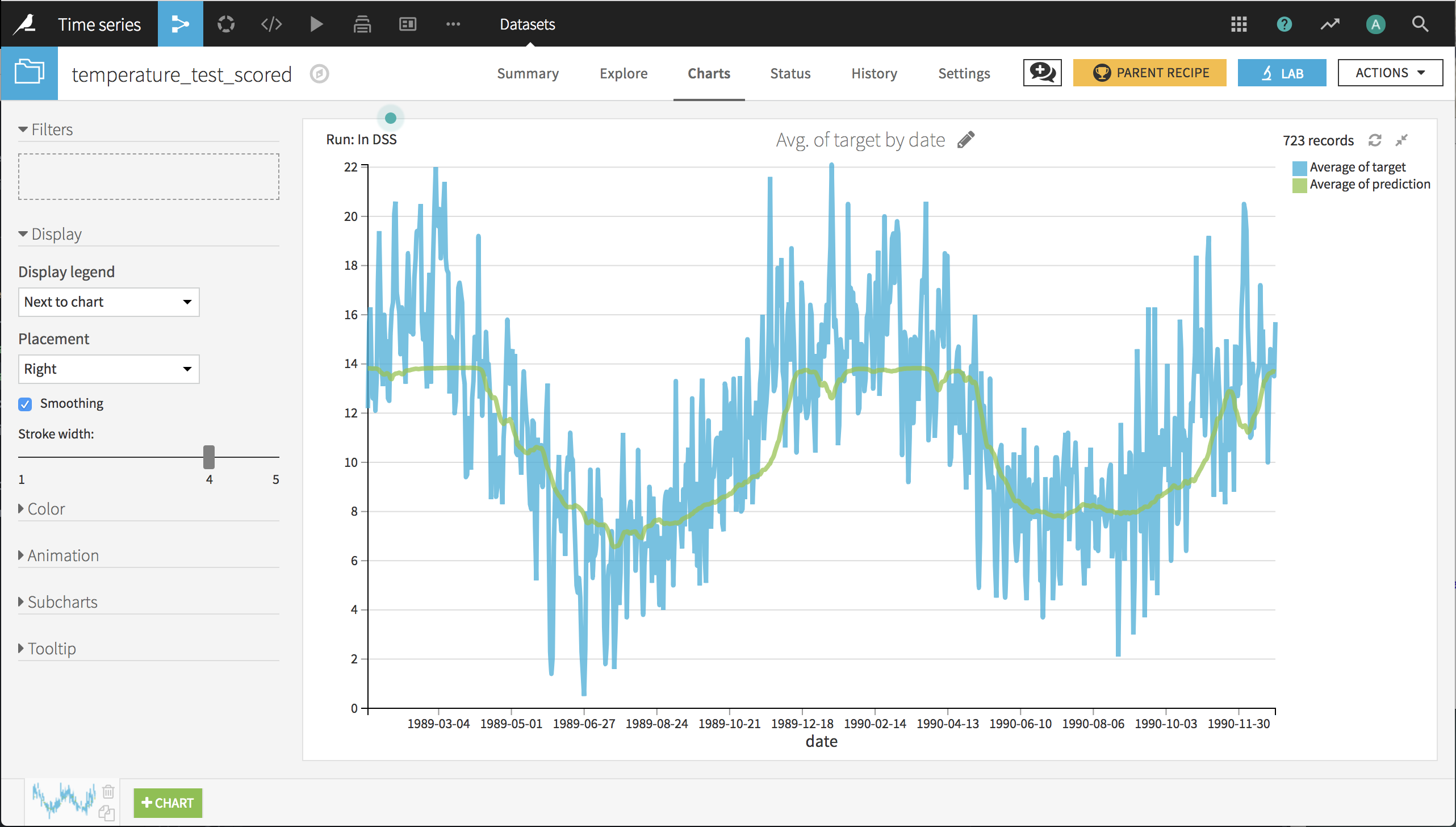
Click Train and, when complete, deploy this model in the flow and score it on the test set. In the scored dataset, create a basic line chart of the temperatures by date, and you can see the model managed to pick up the general trend. It does not perfectly fit the curve, because it is generalizing. The minimum temperature in a country as vast as Australia can fluctuate a lot in a pseudo-random fashion.

Wrap Up
See a completed version of this project on the Dataiku gallery.
See the Dataiku DSS reference documentation on deep learning.