Perform Exploratory Data Analysis (EDA) Using Code Notebooks

Sometimes it’s difficult to spot broader patterns in the data without doing a time-consuming deep dive. Dataiku DSS provides the tools for understanding data at a glance using advanced exploratory data analysis (EDA).

This section will cover code notebooks in Dataiku DSS and how they provide the flexibility of performing exploratory and experimental work using programming languages such as SQL, SparkSQL, Python, R, Scala, Hive, and Impala in Dataiku DSS.

Tip

In addition to using a Jupyter notebook, Dataiku DSS offers integrations with other popular Integrated Development Environments (IDEs) such as Visual Studio Code, PyCharm, Sublime Text 3, and RStudio.

Use a Predefined Code Notebook to Perform EDA

• Open the customers_web_joined dataset to explore it.

Notice that the training and testing data are combined in this dataset, with missing revenue values for the “testing” data. We’ll be interested in predicting whether the customers in the “testing” data are high-value or not, based on their revenue.

Let’s perform some statistical analysis on the customers_web_joined dataset by using a predefined Python notebook.

• Return to the Flow.

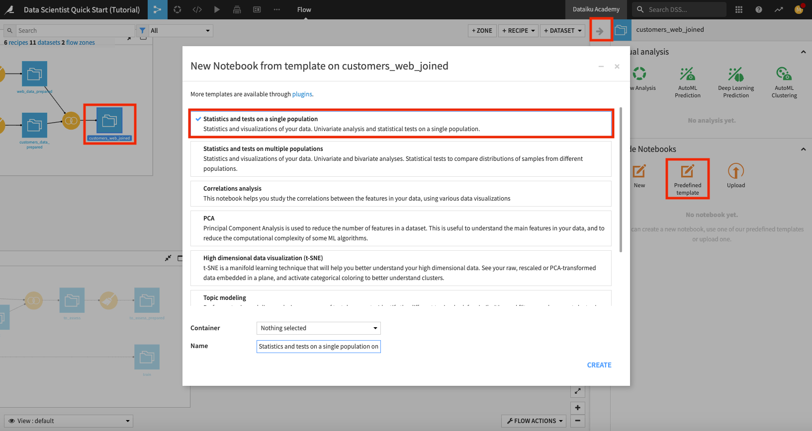
• In the Data preparation Flow Zone, click the customers_web_joined dataset once to select it, then click the left arrow at the top right corner of the page to open the right panel.

• Click Lab to view available actions.

• In the “Code Notebooks” section, select Predefined template.

• In the “New Notebook” window, select Statistics and tests on a single population.

• Rename the notebook to “statistical analysis of customers_web_joined” and click Create.

Dataiku DSS opens up a Jupyter notebook that is prepopulated with code for statistical analysis.

Warning

The predefined Python notebooks in Dataiku DSS are written in Python 2. If your notebook’s kernel uses Python 3, you’ll have to modify the code in the notebook to be compatible with Python 3. Alternatively, if you have a code environment on your instance that uses Python 2, feel free to change the notebook’s kernel to use the Python 2 environment.

Note

Dataiku DSS allows you to create an arbitrary number of Code environments to address managing dependencies and versions when writing code in R and Python. Code environments in Dataiku DSS are similar to the Python virtual environments. In each location where you can run Python or R code (e.g., code recipes, notebooks, and when performing visual machine learning/deep learning) in your project, you can select which code environment to use.

See Setting a Code Environment for details on how to set up Python and R environments and use them in Dataiku DSS objects.

In this notebook, we’ll make the following code modifications:

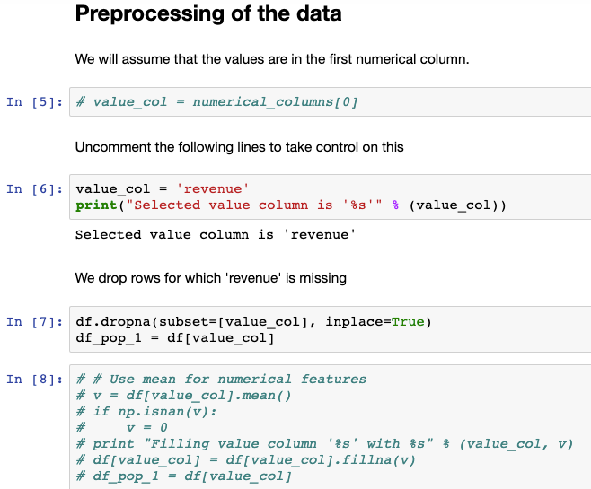
• Go to the “Preprocessing of the data“ section in the notebook and specify the revenue column to be used for the analysis.

• Instead of imputing missing values for revenue, drop the rows for which revenue is empty (that is, drop the “testing” data rows).

• Enclose all the print statements in the notebook in parenthesis for compatibility with Python 3.

The following figure shows these changes for the “Preprocessing of the data“ section in the notebook.

You can make these code modifications in your code notebook, or you can select the pre-made final_statistical analysis of customers_web_joined notebook to see the final result of performing these modifications. To find the pre-made notebook:

• Click the code icon (</>) in the top navigation bar to open up the “Notebooks” page that lists all the notebooks in your project.

Tip

You can also create notebooks directly from the Notebooks page by using the + New Notebook button.

• Click to open the final_statistical analysis of customers_web_joined notebook.

• Run all the cells to see the notebook’s outputs.

Similarly, you can perform a correlation analysis on the customers_web_joined dataset by selecting the Correlations analysis predefined template from the Lab. You can also see the result of the correlation analysis by viewing the project’s pre-made correlation analysis notebook. To do so,

• Open the final_correlation analysis of customers_web_joined notebook from the notebooks page.

• Run the cells of the pre-made notebook.

Notice that revenue is correlated only with the price_first_item_purchased column. There are also other charts that show scatter matrices etc.

You should also explore the buttons at the top of the notebook to see some of the additional useful notebook features.

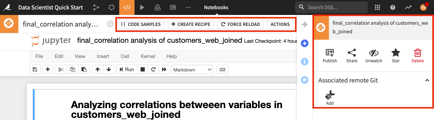
For example, the Code Samples button gives you access to some inbuilt code snippets that you can copy and paste into the notebook, as well as the ability to add your own code snippets; the Create Recipe button allows you to convert a notebook to a code recipe (we’ll demonstrate this in the next section), and the Actions button opens up a panel with shortcuts for you to publish your notebook to dashboards that can be visible to team members, sync your notebook to a remote Git repository, and more.

Tip

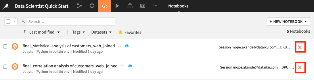
When you’re done exploring the notebooks used in this section, remember to unload them so that you can free up RAM. You can do this by going to the Notebooks page and clicking the “X” next to a notebook’s name.