Customize the Design of Your Predictive Model Using Visual ML

The process of building and iterating a machine learning model using code can quickly become tedious. Besides, keeping track of the results of each experiment when iterating can quickly become complex. The visual machine learning tool in Dataiku DSS simplifies the process of remembering the feature selection and model parameters alongside performance metrics so that you can easily compare models side-by-side and reproduce model results.

This section will explore how you can leverage this visual machine learning tool to perform custom machine learning. Specifically, we’ll discover how to:

• Train several machine learning models in just a few steps;

• Customize preprocessing and model design using either code or the visual interface;

• Assess model quality using built-in performance metrics;

• Deploy models to the Flow for scoring with test datasets; and so much more.

Train Machine Learning Models in the Visual ML Tool

Here, we’ll show various ways to implement the same custom random forest classifier that we manually coded in the Python notebook (in the previous section). We’ll also implement some other custom models to compare their performance.

• Select the train dataset in the Model assessment Flow Zone.

• Open the right panel and click Lab.

• Select AutoML Prediction from the “Visual analysis” options.

• In the window that pops up, select high_value as the feature on which to create the model.

• Click the box for Interpretable Models for Business Analysts.

• Name the analysis high value prediction and click Create.

Note

When creating a predictive model, Dataiku allows you to create your model using AutoML or Expert mode.

In the AutoML mode, DSS optimizes the model design for you and allows you to choose from a selection of model types. You can later modify the design choices and even write custom Python models to use during training.

In the Expert mode, you’ll have full control over the details of your model by creating the architecture of your deep learning models, choosing the specific algorithms to use, writing your estimator in Python or Scala, and more.

It is worth noting that Dataiku DSS does not come with its own custom algorithms. Instead, DSS integrates well-known machine learning libraries such as Scikit Learn, XGBoost, MLlib, Keras, and Tensor Flow.

• Click the Design tab to customize the design. Here, you can go through the panels on the left side of the page to view their details.

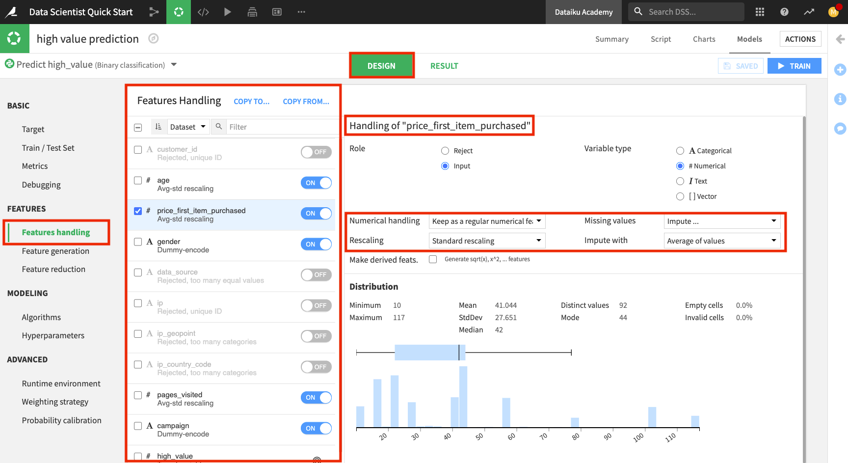
• Click the Features handling panel to view the preprocessing.

Notice that Dataiku has rejected a subset of these features that won’t be useful for modeling. For the enabled features, Dataiku already implemented some preprocessing:

• For the numerical features: Imputing the missing values with the mean and performing standard rescaling

• For the categorical features: Dummy-encoding

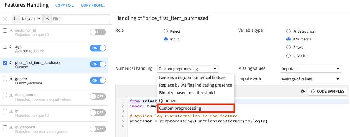
If you prefer, you can customize your preprocessing by selecting Custom preprocessing as the type of “Numerical handling” (for a numerical feature) or “Category handling” (for a categorical feature). This will open up a code editor for you to write code for preprocessing the feature.

• Click the Algorithms panel to switch to modeling.

• Enable Random Forest and disable Decision Tree.

We’ll also create some custom models with code in this ML tool.

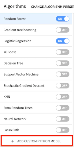
• Click + Add Custom Python Model from the bottom of the models list.

Dataiku DSS displays a code sample to get you started.

Note

The Code Samples button in the editor provides a list of models that can be imported from scikit-learn. You can also write your model using Python code or import a custom ML algorithm that was defined in the project library. Note that the code must follow some constraints depending on the backend you have chosen (in-memory or MLlib).

Here, we are using the Python in-memory backend. Therefore, the custom code must implement a classifier that has the same methods as a classifier in scikit-learn; that is, it must provide the methods fit(), predict(), and predict_proba() when they make sense.

The Academy course on Custom Models in Visual ML covers how to add and optimize custom Python models in greater detail.

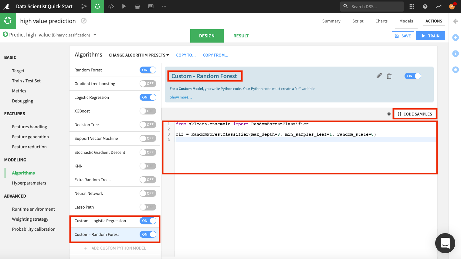
• Click the pencil icon to rename “Custom Python model” to Custom - Logistic Regression.

• Delete the code in the editor and click Code Samples.

• Select Logistic regression and click + Insert.

• Add another custom model. This time, rename the model to Custom - Random Forest.

• Delete the code in the editor and type:

from sklearn.ensemble import RandomForestClassifier
clf = RandomForestClassifier(max_depth=8, min_samples_leaf=1, random_state=0)

• Before leaving this page, explore other panels, such as Hyperparameters, where you can see the “Grid search” strategy being used.

• Also, click the Runtime environment panel to see or change the code environment that is being used.

Tip

The selected code environment must include the packages that you are importing into the Visual ML tool. In our example, we’ve imported libraries from scikit-learn, which is already included in the DSS builtin code environment that is in use.

• Save the changes, then click Train.

• Name the session Customized models and click Train again.

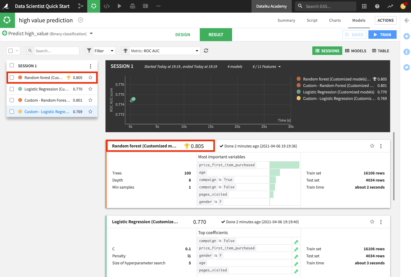
The Result page for the sessions opens up. Here, you can monitor the optimization results of the models for which optimization results are available.

After training the models, the Result page shows the AUC metric for each trained model in this training session, thereby, allowing you to compare performance side by side.

Tip

Every time you train models, the training sessions are saved and listed on the Result page so that you can access the design details and results of the models in each session.

The chart also shows the optimization result for the Logistic Regression model.

Deploy the ML Model to the Flow

Next, we’ll deploy the model with the highest AUC score (the Random forest model) to the Flow to apply it to the test data and evaluate the test data predictions in light of the ground truth classes.

• Click Random forest (Customized model) from the list to go to the model’s Report page.

• Explore the model report’s content by clicking any of the items listed in the left panel of the report page, such as any of the model’s interpretations, performance metrics, and model information.

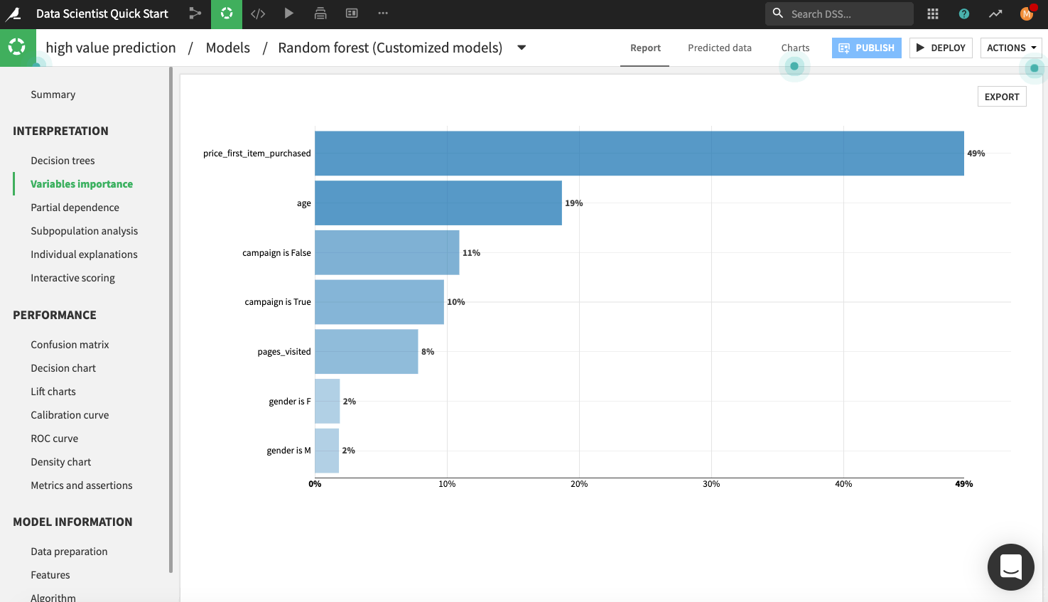
The following figure displays the “Variables importance” plot, which shows the relative importance of the variables used in training the model. Model interpretation features like those found in the visual ML tool can help explain how predictions are made and ensure that fairness requirements around features (such as age and gender) have been met.

Note

You can automatically generate the trained model’s documentation by clicking the Actions button in the top right-hand corner of the page. Here, you can select the option to Export model documentation. This feature can help you easily document the model’s design choices and results for better information sharing with the rest of your team.

Let’s say, overall, we are satisfied with the model. The next thing to do is deploy the model from the Lab to the Flow.

• Click Deploy from the top right corner of the page, and name the model Random Forest.

• Click Create.

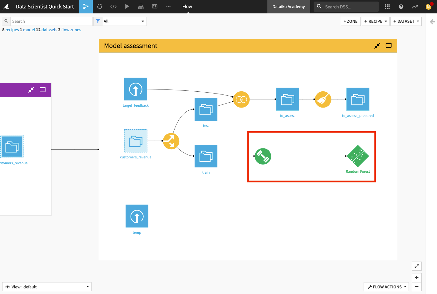
Back in the Flow, you can see that two new objects have been added to the Flow. The green diamond represents the Random Forest model.

Score the ML Model

Now that the model has been deployed to the Flow, we’ll use it to predict new, unseen test data. Performing this prediction is known as Scoring.

• Click the Random Forest model in the Model assessment Flow Zone.

• In the right panel, click Score.

• In the scoring window, specify test as the input dataset.

• Name the output dataset scored and store it in the CSV format.

• Click Create Recipe. This opens up the Settings page.

• Click Run.

• Wait for the job to finish running, then click Explore dataset scored.

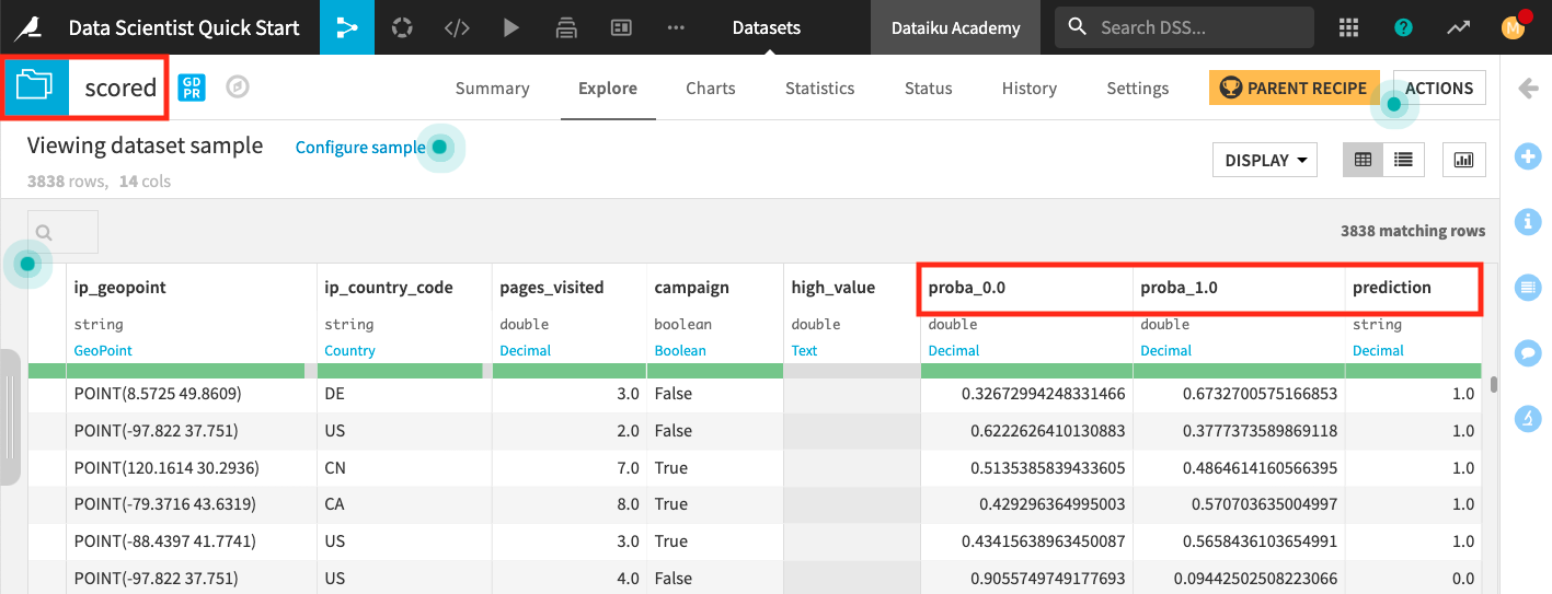
The last three columns of the scored dataset contain the probabilities of prediction and the predicted class.

When you return to the Flow, you’ll see additional icons that represent the Score recipe and the scored dataset.

Evaluate the Model Predictions

For this part, let’s take a look into the Model assessment Flow Zone.

Let’s say that a data analyst colleague created the Flow in this zone so that the to_assess_prepared dataset includes the data for customers in the test dataset and their known classes. We can now use the to_assess_prepared dataset to evaluate the true performance of the deployed model.

We’ll perform the model evaluation as follows.

• Double click the Model assessment Flow Zone to open it.

• Click the to_assess_prepared dataset and open the right panel to select the Evaluate Recipe from the “Other recipes” section.

• Select Random Forest as the “Prediction model”.

• Click Set in the “Outputs” column to create the first output dataset of the recipe.

• Name the dataset Predictions and store in CSV format.

• Click Create Dataset.

• Click Set to create the metrics dataset in a similar manner.

• Click Create Recipe.

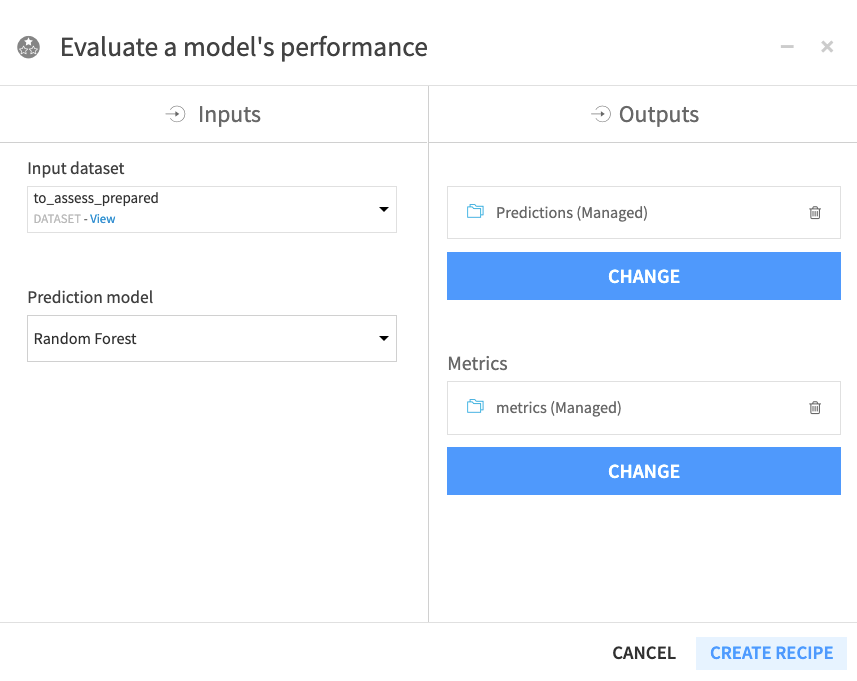
• When the recipe window opens, click Run.

• Return to the Flow to see that the recipe has output two datasets: the metrics dataset, which contains the performance metrics of the model, and the predictions datasets, which contains columns about the predictions.

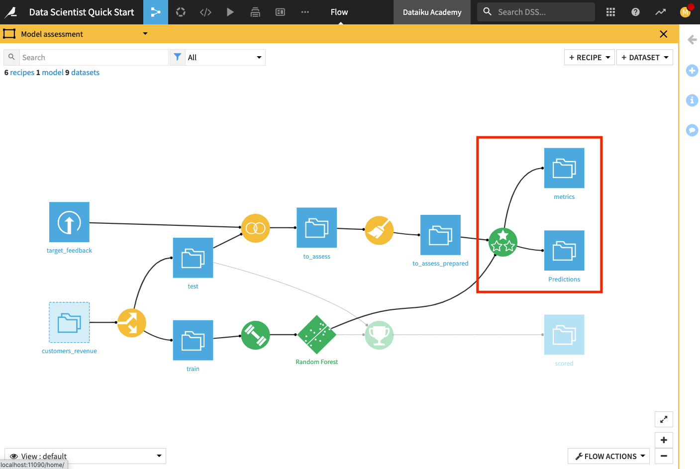
• Open up the metrics dataset to see a row of computed metrics that include the AUC score.

• Return to the Flow and open the Predictions dataset to see the last four columns which contain the model’s prediction of the test dataset.

• Return to the Flow.

Tip

Each time you run the Evaluate recipe, DSS appends a new row of metrics to the metrics dataset.