Solution | Site Selection#

Overview#

Business case#

Site Selection is an AI-powered location intelligence system for expansion strategy. It helps organizations evaluate where to open, expand, rationalize, or optimize physical service locations in contexts where location decisions directly affect customer reach, revenue capture, service accessibility, competitive positioning, and capital allocation.

The solution combines geospatial analytics, drive-time catchment analysis, demographic enrichment, competition and cannibalization measurement, and a transparent Opportunity Score to support location decisions. Its main objective is to answer the question: which candidate locations offer the strongest balance of demand, competitive attractiveness, and white-space opportunity?

This solution doesn’t replace final real-estate due diligence. It’s intended to prioritize and explain candidate locations before deeper validation using lease cost, zoning, operational feasibility, legal constraints, brand strategy, and field knowledge.

Installation#

From the Design homepage of a Dataiku instance connected to the internet, click + Dataiku Solutions.
Search for and select Site Selection.
If needed, change the folder into which the Solution will be installed, and click Install.
Follow the modal to either install the technical prerequisites below or request an admin to do it for you.

Note

Alternatively, download the Solution’s .zip project file, and import it to your Dataiku instance as a new project.

Technical requirements#

To use this Solution, you must meet the following requirements:

Have access to a Dataiku 14.5+* instance.
Have the Geo Router plugin version 1.2.2 installed and configured.
Have the Agent Hub plugin configured and available for the Site Selection Assistant.
Have a Python 3.10 code environment named solution_site-selection.
Have an SQL connection available through Project Setup. In the packaged solution, this is configured through the project variable main_connection.
Have a compatible filesystem connection for managed folders, configured through the project variable folders_connection.
Have an LLM connection available through Project Setup for the assistant and knowledge retrieval configuration.

The required Python packages are:

fiona
geopandas
h3
joblib
matplotlib
pyarrow
pyproj
rtree
scikit-learn
scipy
shapely
tqdm

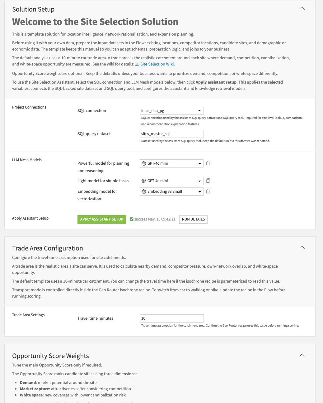
The project is designed to be configured through Project Setup so that users can adapt the solution to their own execution environment without editing recipes manually. Project Setup is used to configure connection names, scoring parameters, travel-time assumptions, assistant configuration, tool identifiers, and Knowledge Base identifiers before running the solution.

Data requirements#

The Solution is shipped with synthetically generated data relevant to a location intelligence and expansion planning use case.

The input data has four already prepared datasets covering existing sites, competitor sites, candidate locations, and demographic or economic context:

Dataset	Description
own_stores_info	Includes existing company locations used to measure current network coverage, performance context, and cannibalization risk.
competition_info	Includes competitor locations used to measure competitive pressure and market saturation.
candidates_info	Includes potential new sites to evaluate and rank.
demography_info	Includes population, household, income, and optional economic indicators used to estimate demand strength.

The three site datasets, own_stores_info, competition_info, and candidates_info, must contain valid latitude and longitude fields because they’re used to create GeoPoints and drive-time isochrones.

The demography_info dataset must contain valid polygon geometry because it’s used to enrich each site catchment with population, income, household, and economic context.

Detailed field expectations#

own_stores_info

store_id: mandatory unique identifier for each existing owned location.
lat, lon: mandatory latitude and longitude used to create the site GeoPoint.
avg_monthly_revenue: optional performance metric used for dashboard interpretation.
avg_number_customers: optional customer volume metric used for business context.
store_category: optional store format or category, such as express, standard, or flagship.
store_open_date: optional opening date used for network maturity or context.

Granularity: one row per existing owned store, branch, ATM, clinic, or service location.

competition_info

comp_id: mandatory unique identifier for each competitor location.
lat, lon: mandatory latitude and longitude used to create the GeoPoint.
comp_category: optional competitor category or type.
Brand: optional competitor brand name.

Granularity: one row per competitor location.

candidates_info

cand_site_id: mandatory unique identifier for each candidate site.
lat, lon: mandatory latitude and longitude used to create the GeoPoint.
cand_category: optional candidate site format or category.

Granularity: one row per candidate site.

demography_info

Location_id: mandatory unique identifier for each geographic area.
polygon: mandatory geometry representing the area.
total_population: mandatory population size.
median_household_income: mandatory purchasing power indicator.
number of households: mandatory stability or repeat-demand indicator.
population_males: optional demographic split.
population_females: optional demographic split.
median_age: optional age profile.
avg rent: optional affordability signal.
avg_property_price: optional economic strength signal.
business_establishment_count: optional business activity indicator.
retail_poi_count: optional retail density indicator.
office_poi_count: optional workplace density indicator.

Granularity: one row per census, geographic, or market polygon.

Workflow overview#

You can follow along with the Solution in the Dataiku gallery.

The project has the following high-level steps:

Prepare your input datasets according to the expected data model.
Open Project Setup and configure the required project variables, including connection names, travel-time assumption, scoring weights, agent IDs, tool IDs, and Knowledge Base IDs.
Load or connect the required datasets: own stores, competitor sites, candidate sites, and census, demographic, or economic data.
Run the pipeline from the first to the last Flow zone.
Review dashboard outputs such as candidate ranking, opportunity score distribution, demand strength, competition pressure, and white-space or cannibalization indicators.
Use the Site Selection Assistant to ask questions about metrics, candidate sites, score logic, and business interpretation.
Validate the highest-ranked sites with business, real-estate, finance, and operations teams before making investment decisions.

Walkthrough#

Note

In addition to reading this document, it’s recommended to read the wiki of the project before beginning to get a deeper technical understanding of how this Solution was created and more detailed explanations of Solution-specific vocabulary.

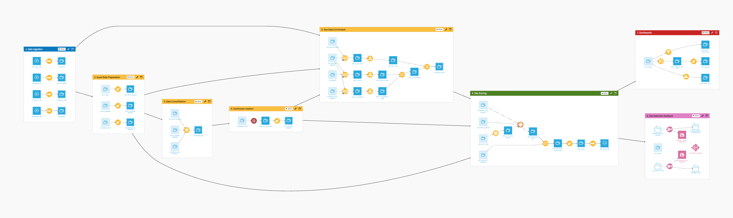
The Flow is organized into 8 modular zones:

Data Ingestion
Input Data Preparation
Data Consolidation
Isochrone Creation
Geo Data Enrichment
Site Scoring
Site Selection Visualization
Site Selection Assistant

Prepare and plug your data#

This Solution follows a template-based approach: data must first be prepared externally to match the expected input schema, then loaded into the project Flow.

The Flow is divided into multiple Flow zones, each dedicated to a specific stage of the site selection pipeline. Detailed explanations for each Flow zone can be found in the project wiki. Below is a high-level overview of the major tasks.

The ingestion layer is designed for schema consistency, reproducibility, and compatibility with SQL execution. The packaged project uses Project Setup variables for connection names and configuration values so the same solution can be reused across different deployments with fewer manual changes.

Clean and prepare location data#

The Solution organizes data preparation into dedicated Flow zones to ensure that location, competition, demand, and scoring inputs are structured consistently:

Data Ingestion: collects the four core input datasets: own stores, competitor sites, candidate sites, and demographic or economic polygons.
Input Data Preparation: standardizes own stores, candidates, and competitors into a unified structure by creating geospatial fields, aligning identifiers, and introducing a common site classification through site_role.
Data Consolidation: combines the standardized site datasets into a single dataset named consolidated_sites so downstream geospatial computations can run on one common structure.
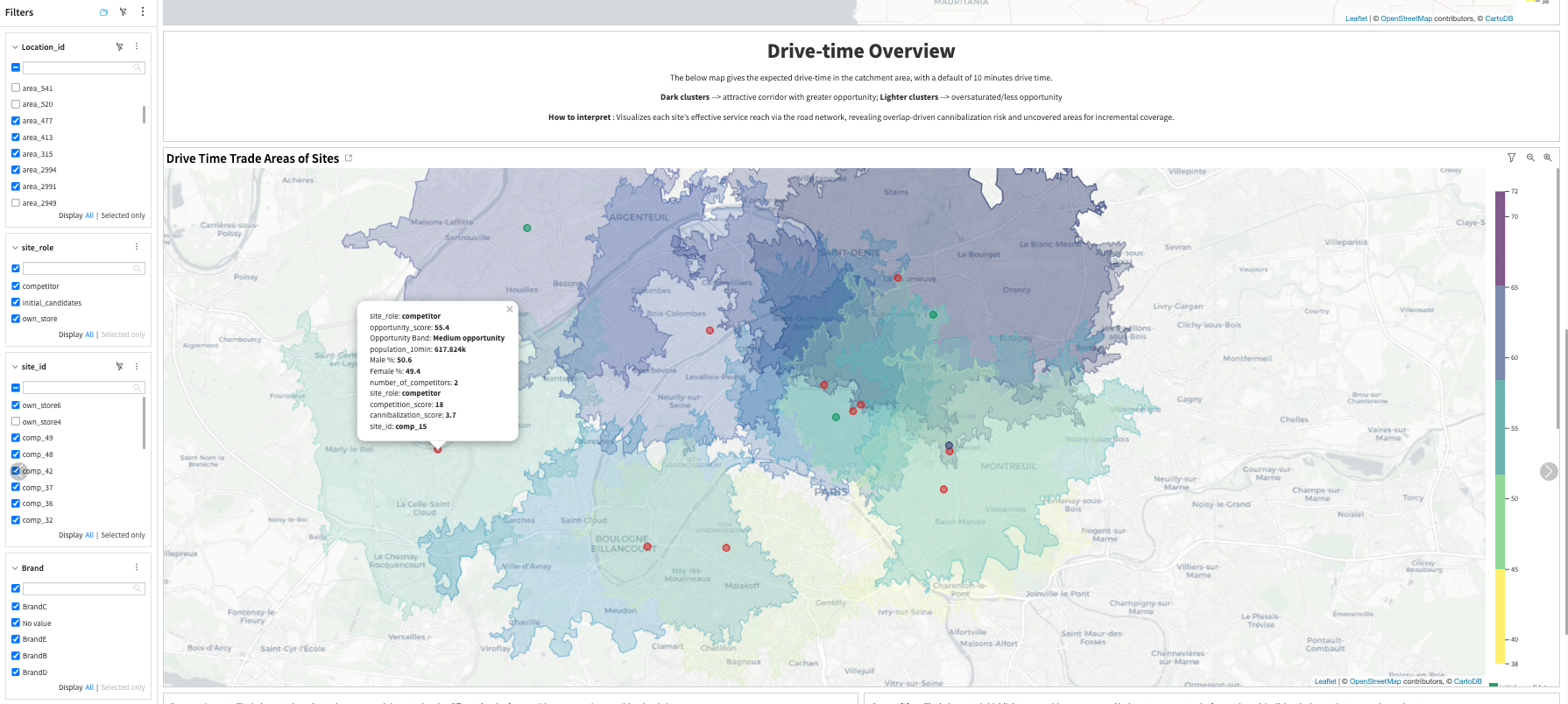
Isochrone Creation: generates travel-time catchment polygons around each site. The default example uses 10-minute drive-time catchments, and the travel-time value can be configured through Project Setup.
Geo Data Enrichment: enriches each catchment with demand, competition, and own-network overlap features using geospatial joins, aggregations, and feature engineering.
Site Scoring: converts enriched features into interpretable sub-scores and a final Opportunity Score from 0 to 100. You can update scoring weights and parameters through Project Setup to reflect different business strategies or industry contexts.
Site Selection Visualization: creates the visualizations and dashboard-ready datasets used by business users.
Site Selection Assistant: supports the conversational AI layer that explains metrics, compares sites, and provides decision support. The assistant relies on different knowledge bases, Agent tools, where SQL tool is required to be configured through Project Setup.

Create site catchments with isochrones#

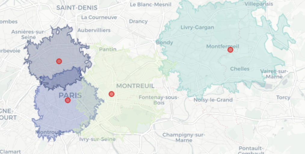
An isochrone is a geographic polygon representing all locations that can be reached from a starting point within a defined amount of time, based on a transportation mode and the underlying road or travel network.

This step is central because downstream calculations are performed inside these catchments:

Demand depends on how much population, income, and household volume falls inside the isochrone.
Competition pressure depends on how many competitors exist inside the same accessible area.
Cannibalization depends on how much overlap exists between candidate-site catchments and owned-store catchments.

The packaged solution uses a 10-minute drive-time catchment as the default example. This assumption can be changed through Project Setup, allowing users to adapt the solution to different industries or market contexts. For example, a 5 to 10 minute walking catchment may fit dense urban use cases, while a 10 minute driving catchment may be more realistic in suburban contexts, and a 15 to 20 minute catchment may better fit destination services such as healthcare.

Enrich sites with demand, competition, and cannibalization signals#

The enrichment zone converts spatial relationships into numerical site-level features.

Own-store overlap is measured by joining site isochrones with owned-store locations and counting distinct owned stores inside each isochrone. Demand enrichment is performed by intersecting isochrones with census or demographic polygons and aggregating attributes such as population, households, income, and economic indicators. Competition enrichment is performed by locating competitor points inside each site catchment and aggregating competition counts and related indicators.

The enriched demand, competition, and cannibalization features are then consolidated into a single scoring input table.

Score and prioritize candidate sites#

The scoring layer is deterministic, transparent, and configurable rather than a black-box machine learning model. You can configure these scores through Project Setup; additional technical details are available in the project wiki. Scoring combines three primary decision dimensions:

Demand strength: is there enough market potential around the site?
Market capture: can the site realistically capture demand in the presence of competitors?
White-space opportunity: does the site expand coverage without heavily cannibalizing the existing network?

The final Opportunity Score is built from those components and scaled to a 0 to 100 range.

Demand score#

The demand score combines normalized population, income, and household indicators.

demand = W_POP * population + W_INC * income + W_HH * households

Default demand weights are:

W_POP = 0.55
W_INC = 0.25
W_HH = 0.20

These weights are configurable through Project Setup. Users can adjust them when the business wants to emphasize a different interpretation of demand. For example, a grocery or essential retail use case may emphasize population and households, while a premium retail use case may assign more importance to income.

Competition pressure#

The competition logic uses a Huff-inspired but simplified approach. Instead of full probabilistic demand allocation, it estimates competitive pressure based on nearest competitor proximity and competitor density.

Default competition parameters are:

W_NEAREST = 0.70
W_DENSITY = 0.30
LAMBDA = 2.0

The interpretation is:

Competition density measures the total number of competitors in the catchment.
Nearest competitor impact measures the influence of the closest competitor.
Competition score is calculated so that higher competitive pressure lowers the attractiveness of the site.

White space and cannibalization#

Cannibalization is measured using the number of owned stores in the catchment and the distance to the nearest owned store.

cannibalization = W_OWN_COUNT * own_store_count + W_OWN_DISTANCE * proximity
white_space = 1 - cannibalization

High white space suggests untapped demand, while low white space suggests that demand may shift from existing stores.

This is useful because cannibalization tolerance changes by industry. For example, coffee chains and convenience retail may tolerate denser store networks, while banking branches, clinics, and destination retail may require larger separation between locations.

Final Opportunity Score#

The final opportunity score combines demand, competition-adjusted market attractiveness, and white-space opportunity.

opportunity = ALPHA_DEMAND * demand + ALPHA_COMP * market_share + ALPHA_WHITE * white_space

Default final weights are:

ALPHA_DEMAND = 0.55
ALPHA_COMP = 0.30
ALPHA_WHITE = 0.15

These default weights are configured through Project Setup. Users can modify them to reflect different business strategies, provided the alpha weights continue to sum to 1.0.

Typical tuning examples include:

Increase demand weight when prioritizing high-demand areas.
Increase competition penalty when avoiding crowded markets.
Increase cannibalization penalty when avoiding overlap with existing stores.
Reduce distance sensitivity when customers are willing to travel farther.
Reduce the white-space penalty for more aggressive expansion strategies.

Site Selection dashboards#

The Site Selection dashboards provide a decision-oriented view of market attractiveness, location-level opportunity, and expansion prioritization.

Page	Description
Summary	Provides an executive-level view of the overall market landscape, including number of sites, operational sites, competition intensity, white space, average opportunity score, and opportunity tier distribution.
Network Competition Proximity	Shows distance-based diagnostics to understand how candidate sites relate to the existing network and to nearby competitors.
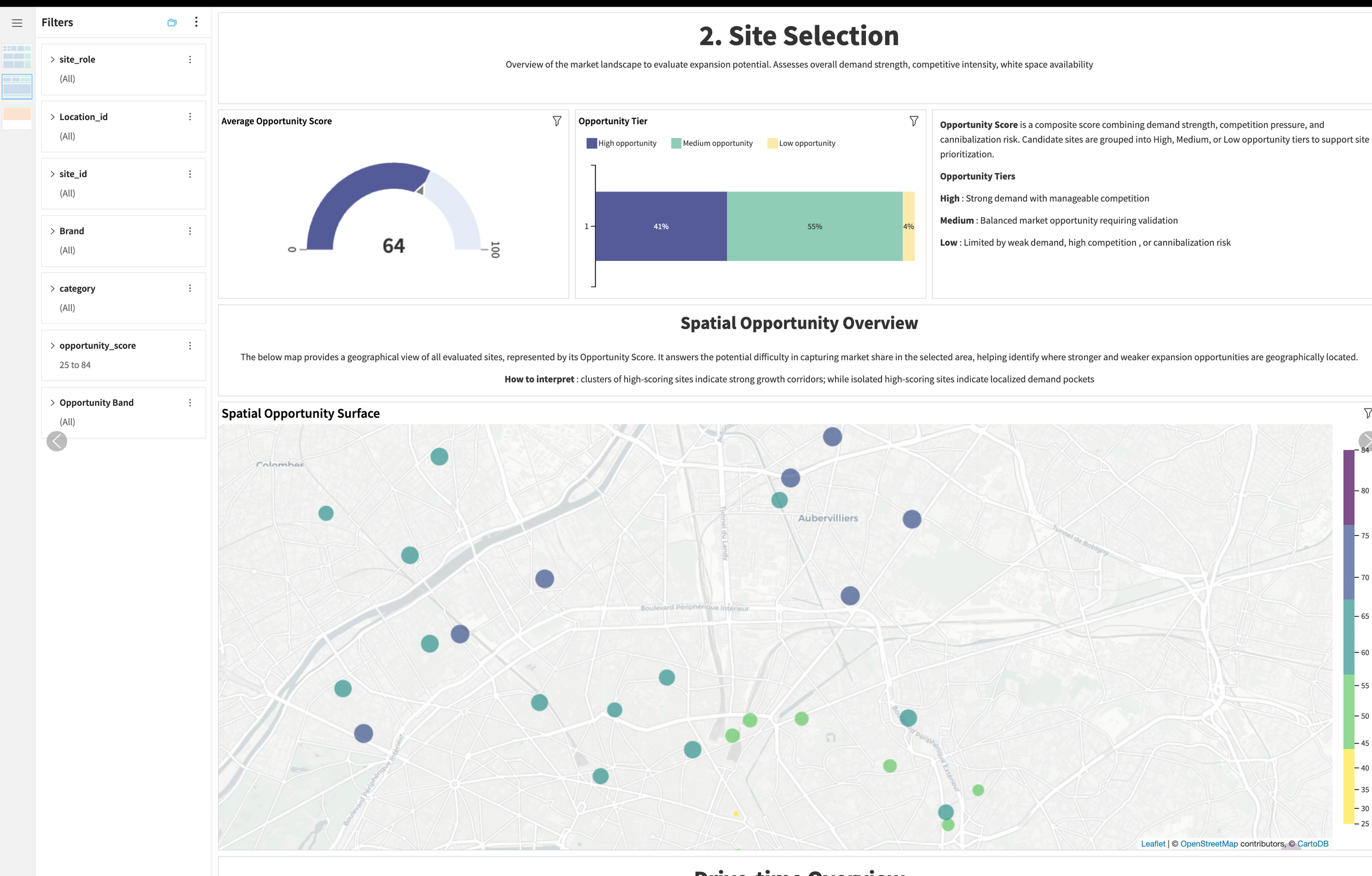
Site Selection	Provides the location-level decision layer, including spatial views of opportunity score, opportunity tier, and travel-time catchments.
Market Performance Analysis	Explains performance drivers by comparing revenue, demand, competitor density, and opportunity score.
Site Ranking	Provides the final ranked list of sites for shortlisting and prioritization.
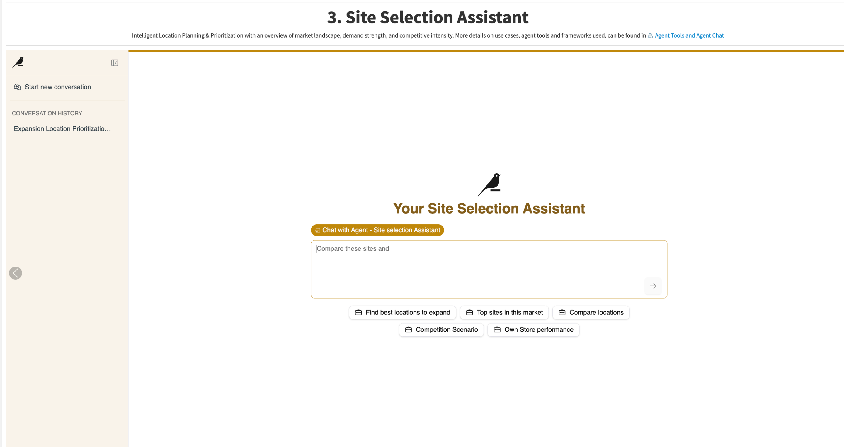
Site Selection Assistant	Provides a conversational interface to ask questions about candidate sites, metrics, score logic, and business recommendations.

The dashboard supports a natural decision flow: start with Summary, move to Site Selection, then use Performance Analysis to understand drivers, use Site Ranking to finalize shortlists, and use the Assistant to go deeper or explain decisions.

Filters allow users to focus the dashboard on a specific decision context. For example, users can filter by site role, candidate tier, location, market area, or opportunity band. This helps the same dashboard support different business questions such as expansion prioritization, competitive analysis, white-space identification, and network rationalization.

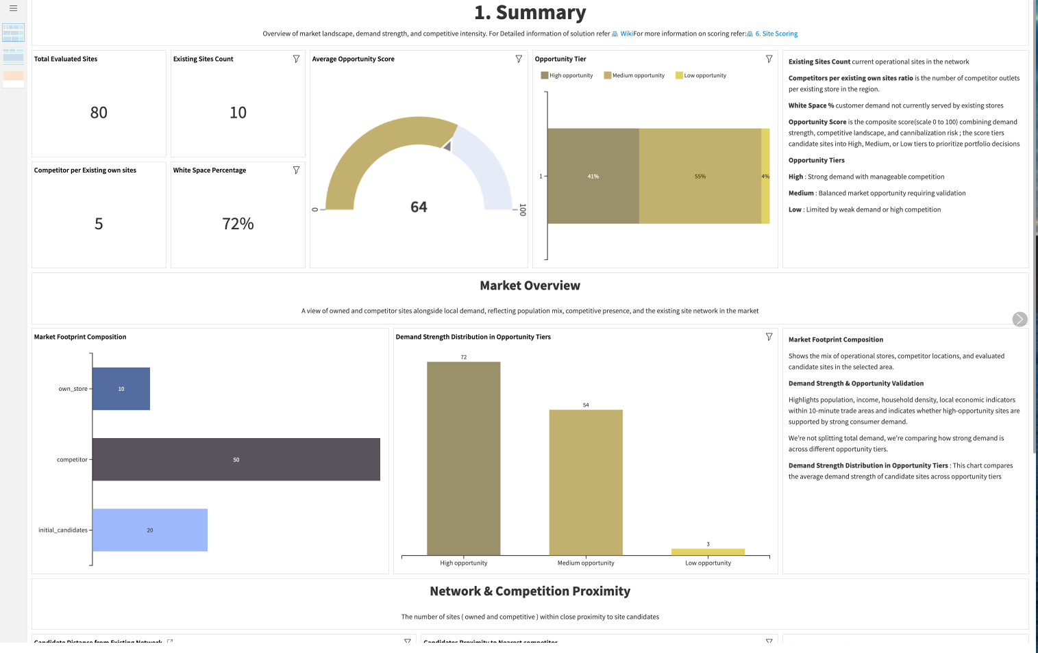
Summary page#

The Summary dashboard gives business users an executive-level overview of the site selection landscape. It helps users understand the number of locations being analyzed, the balance between owned stores, competitors, and candidate sites, and the overall distribution of opportunity across the market.

This dashboard shows:

Total number of sites in the analysis
Number of operational or existing owned locations
Competition intensity across the market
Average opportunity score
White-space indicators
Distribution of candidate sites by opportunity tier
Candidate proximity to the nearest competitor
Candidate proximity to the nearest owned store

Site Selection page#

The Site Selection Page is the core location decision page. It combines maps, catchment areas, opportunity scores, and tiers to help users identify which candidate locations should be prioritized.

This dashboard shows:

Candidate sites by opportunity score
Candidate sites by opportunity tier: High, Medium, and Low
Drive-time catchment polygons
Spatial overlap with competitors and owned stores
White-space areas and high-potential market pockets
Location-level metrics that explain why a site is attractive or risky
Own Store Revenue versus demand indicators
Competitor density versus opportunity score
Demand strength across market areas
Ranked candidate sites by Opportunity Score

Site Selection Assistant#

The Site Selection Assistant is built with Dataiku Agent Hub and Agent Chat. It provides a conversational AI layer for site selection decision support.

The assistant is intended to:

Identify high-potential locations
Explain why a site is recommended
Compare alternatives
Interpret scoring metrics
Incorporate economic context
Translate scoring outputs into business-ready recommendations

The assistant relies on configured tools and knowledge bases rather than free-form generation alone. Its role is to retrieve site facts, compare sites, explain metrics, and translate scoring outputs into business-friendly explanations.

Agent tools#

Tool	Type	Purpose
Get Site Profile	Dataset Lookup	Retrieves structured data for a specific site, including opportunity score, demand, competition, cannibalization, white space, distance metrics, and demographic indicators.
Compare Sites	Query / Ranking	Ranks and compares multiple sites using consistent scoring logic, with opportunity_score as the default ranking metric.
Explain Site Recommendation	Python	Converts site metrics into a structured business recommendation with strengths, risks, trade-offs, and implications.
Explain Metric	Knowledge Base / RAG	Explains the meaning and interpretation of metrics used in scoring.
Economic Context Retrieval	Knowledge Base / RAG	Provides regional economic context such as commercial activity indicators, business density, affluence proxies, and economic patterns.

The tool and Knowledge Base identifiers are configured through Project Setup. This allows the packaged solution to point to the correct Agent Hub assets after deployment without requiring users to manually update every assistant or recipe reference.

A typical Agent Chat flow is:

Compare sites to identify top candidates.
Retrieve the detailed site profile.
Generate an explanation or recommendation.
Return a structured business-ready answer.

Example questions include:

Which candidate sites should we prioritize for expansion?
Why is cand_site_13 recommended?
Compare the top candidate sites in area_1600.
Which locations have high demand but low competition?
Which candidate sites have high cannibalization risk?
Explain how the Opportunity Score is calculated.

Adaptability across industries#

The Site Selection Solution is industry-flexible because it’s built around a simple structure of sites, catchments, demand, competition, and network overlap. This makes it possible to adapt the same framework across multiple industries by remapping inputs and adjusting scoring assumptions.

Industry vertical	Site entity	Demand drivers	Competitive factors	Cannibalization risks
Retail	Physical store	Population size and household income	Nearby competitor stores	Overlap with existing company stores
Banking	Branch or ATM	Household density and income levels	Other branches or financial access points	Overlap with existing network branches
QSR & Food Chains	Restaurant location	Population size and footfall proxies	Nearby restaurants	Overlap with existing brand outlets
Healthcare	Clinic or service center	Population size and demographic age profile	Nearby medical clinics	Overlap with existing healthcare locations
Logistics & Delivery	Hub, dark store, or pickup point	Household volume or delivery density	Alternative fulfillment points	Overlap with existing delivery service zones

The recipes and pipelines remain largely unchanged; only the data mapping, travel-time assumption, scoring weights, and business interpretation shift as per business requirements.

Reproduce with minimal effort for your data#

This Solution helps users evaluate and prioritize physical locations in Dataiku—from geospatial data preparation to scoring, visualization, and assistant-driven explanation.

This guide outlines multiple ways to derive value. The best setup depends on your data, industry, and site selection objective.

Legal#

Legal disclaimer on demo data#

This solution uses manually generated data and Dataiku makes no representations or warranties regarding the performance, availability, or results that may be obtained from using its business solutions, including with customer data. Use of the solution is at the user’s own risk.

Agent Warning#

The solution is an AI-powered tool intended to support analysis and interpretation only. Responses depend on the accuracy of underlying data, scoring outputs, and configured knowledge bases. All agent outputs must be reviewed by a qualified stakeholder before being used to support investment decisions.

Responsible AI considerations#

The Site Selection solution follows a responsible AI approach by ensuring that recommendations are transparent, explainable, and grounded in business signals such as demand, competition, cannibalization, and white space. It’s designed to support decision-making rather than replace it.

The responsible AI considerations are:

Only appropriate, non-sensitive data should be used.
Inputs are expected to be accurate, current, and compliant with data-governance standards.
The scoring logic is applied consistently across locations to avoid bias.
Economic context is used as a supporting signal, not as the only decision criterion.
Final decisions should still consider real-world factors such as cost, regulations, operational constraints, zoning, lease terms, and field knowledge.
Continuous monitoring and periodic validation are needed to keep the solution aligned with business objectives and changing market conditions.
Project Setup values should be reviewed before deployment so that scoring weights, connections, LLM configuration, and assistant references are appropriate for the target environment.
Users should avoid using sensitive personal data unless it’s necessary, lawful, governed, and aligned with organizational data policies.