Solution | Distribution Spatial Footprint#

Overview#

Business case#

Distribution spatial footprint analysis is a powerful way to optimize retail networks depending on customers, competition, and distribution centers locations: this optimization is particularly critical for retailers.

Fueled with the right data, it can generate up to 20% in sales increase. Achieving these results relies on both global and local network optimizations, for which several use cases can be implemented such as opening/closing/relocating stores, finding the best places for new distribution centers, optimizing marketing campaigns based on local networks specificity etc.

A fundamental aspect of this Solution is the computation of isochrone areas to enrich the input data for geospatial analysis. Isochrone areas are a type of catchment area which represents the area from which a location is reachable by someone within a given amount of time, using a particular mode of transportation.

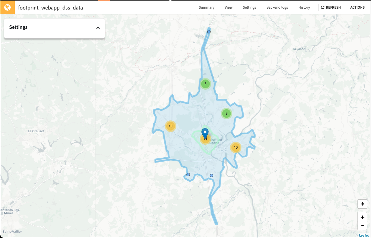
The Solution consists of a data pipeline that computes isochrones areas, further enriches the input data using these computed areas, and in doing so opens up a wide range of geospatial analyses. Analysts can input their own data and surface the outputs in a dashboard or interactive webapp to analyze their organization’s own distribution networks. Data scientists should use this Solution as an initial building block to develop advanced analytics / support decision making. Dataiku can also offer roll-out and customization services on demand.

Installation#

From the Design homepage of a Dataiku instance connected to the internet, click + Dataiku Solutions.
Search for and select Distribution Spatial Footprint.
If needed, change the folder into which the Solution will be installed, and click Install.
Follow the modal to either install the technical prerequisites below or request an admin to do it for you.

Note

Alternatively, download the Solution’s .zip project file, and import it to your Dataiku instance as a new project.

Technical requirements#

To leverage this Solution, you must meet the following requirements:

Have access to a Dataiku 13.3+* instance.
An API key for Openrouteservice or Here, a location platform for developers.
A Python 3.9 code environment named solution_distribution-spatial-footprint with the following required packages:

openrouteservice==2.3.3
folium==0.12.1
geopy==2.1.0
geopandas==0.8.2
Shapely==1.7.1
Flask==1.1.2
flexpolyline==0.1.0
scikit-learn==0.24.2

Install the following plugins:
- Geocoder
- Reverse Geocoding/Admin Maps
- Distribution Footprint Webapp
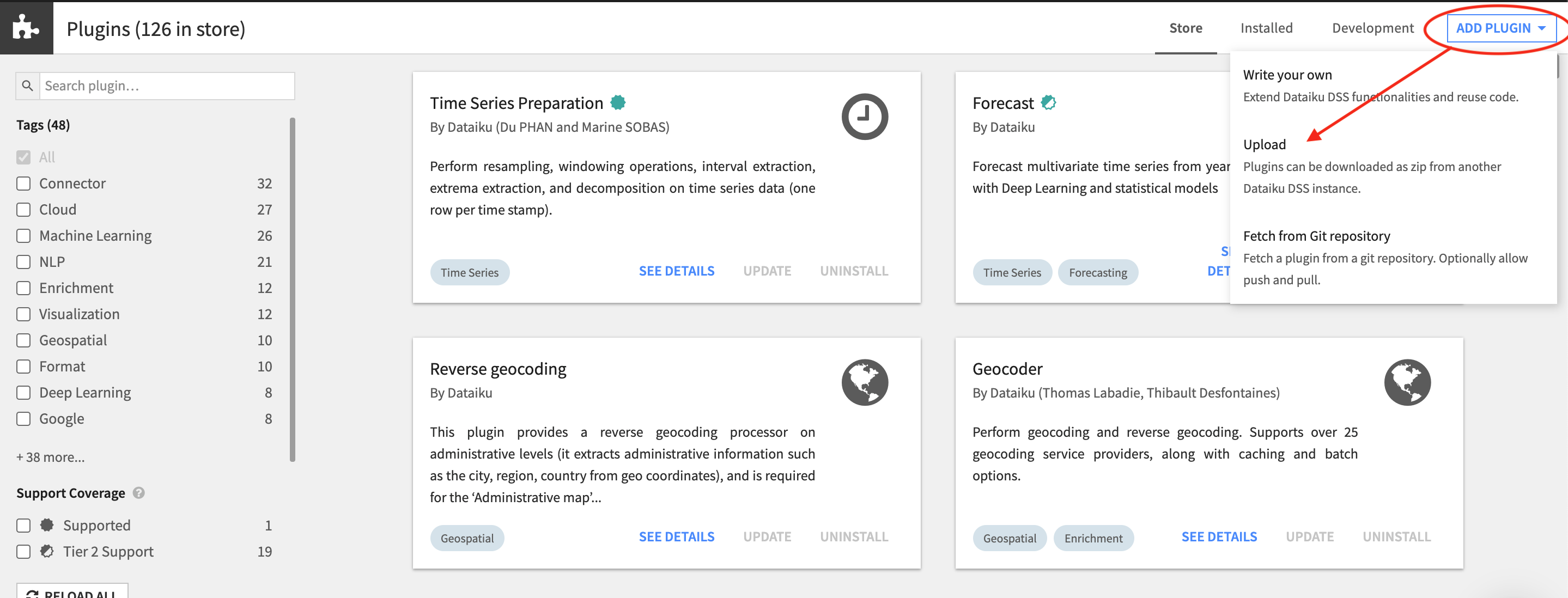
  - To install this custom plugin, select Add Plugin > Upload, and select the zip file. You will be asked to create a Python 3.6 environment for the plugin.
  Note
  
  The webapp requires this plugin, but it’s not necessary for the project, project setup, and dashboards to run.

Data requirements#

The Dataiku Flow was initially built using publicly available data consisting of various French grocery store locations in the Burgundy region of France and fictional customer data.

However, we intend for you to use this project with your own data, which you can upload using the Project Setup. Your input data should meet the general data requirements and will be renamed to the following datasets:

Dataset	Description
locations_dataset	Meets the following data requirements: Dataset Granularity: 1 row = 1 single location. Requirements: The dataset should have at least 1 key (1 column or a column combination) allowing for the identification of each single location. Two columns, exactly named latitude and longitude OR A single address column, exactly named address
customers_dataset (optional)	Meets the following data requirements: Dataset Granularity: 1 row = 1 customer Requirements: The dataset should have a single column allowing to identify each customer named customer_id. Two columns, exactly named latitude and longitude OR A single address column, exactly named address

Dataset

Description

locations_dataset

Meets the following data requirements:

Dataset Granularity: 1 row = 1 single location.
Requirements:
- The dataset should have at least 1 key (1 column or a column combination) allowing for the identification of each single location.
- Two columns, exactly named latitude and longitude OR
- A single address column, exactly named address

customers_dataset (optional)

Meets the following data requirements:

Dataset Granularity: 1 row = 1 customer
Requirements:
- The dataset should have a single column allowing to identify each customer named customer_id.
- Two columns, exactly named latitude and longitude OR
- A single address column, exactly named address

Workflow overview#

You can follow along with the sample project in the Dataiku gallery.

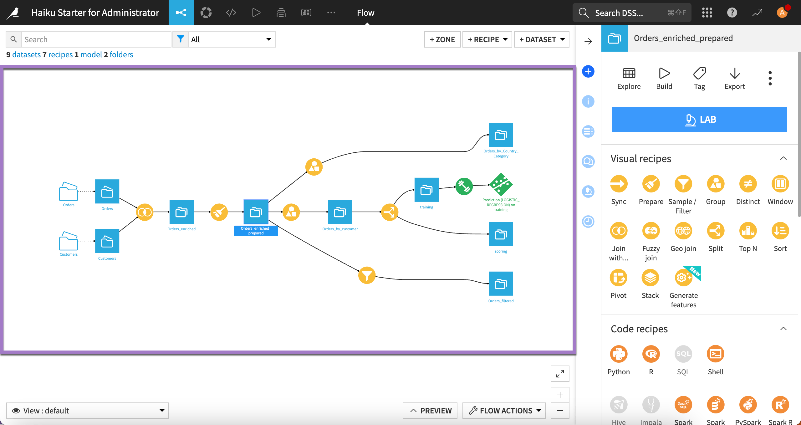
The project has the following high level steps:

Input your data and select your analysis parameters via the Project Setup.
Ingest and pre-process the data to be compatible with geospatial analysis.
Compute requested isochrones per location using the selected API service.
If you’ve provided customer data, identify and count the customers located within your distribution network isochrones.
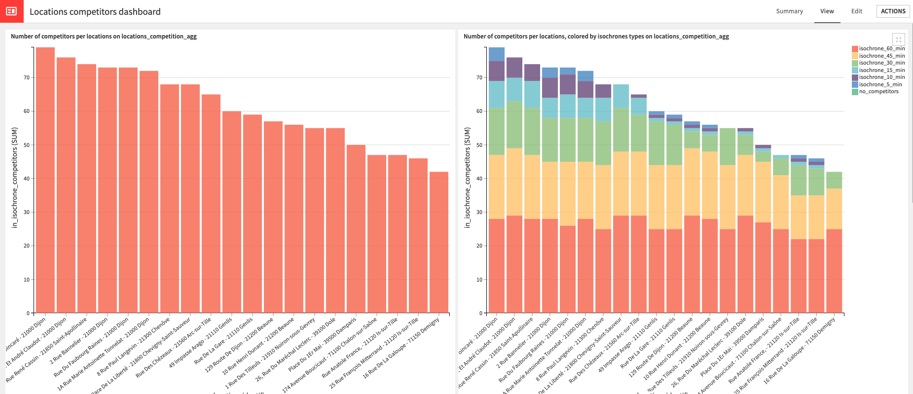
Visualize the overlapping isochrones in your distribution network, as well as the locations of customers (if applicable) using pre-built dashboards.
Interactively analyze your distribution spatial footprint using a pre-built webapp.

Walkthrough#

Note

In addition to reading this document, it’s recommended to read the wiki of the project before beginning to get a deeper technical understanding of how this Solution was created and more detailed explanations of Solution-specific vocabulary.

Plug and play with your own data and parameter choices#

Once you’ve created the new project, you can walk through the steps of the Project Setup to add your data and select the analysis parameters to run.

In the Inputs section of the Project Setup, upload your distribution network dataset and, optionally, customer dataset. Refer to the Data requirements section above for the specific formatting requirements for your data. In this section, you will also need to specify the identifier column or columns (that is, those containing location data) and how your locations are defined (that is, latitude/longitude or addresses). It’s important that you select the location definition as this will impact which preprocessing steps run in the Flow.
Move on to the Isochrones section, where you will be asked to select an API service. At this time you should copy your API key and paste it into the correct field of the App. Here you will also be able to select the mode of transportation to base your isochrones off of, the isochrones to be computed based on travel time from a central location, and any other isochrone attributes of interest. Please note that isochrone attributes may vary between API providers.
Optionally, if you uploaded a customer dataset, the final Customers section of the Project Setup is where you can select which specific isochrones you want to search for customers within.
Once all the data and parameters are setups, you can click the Run Now button to start the full analysis.

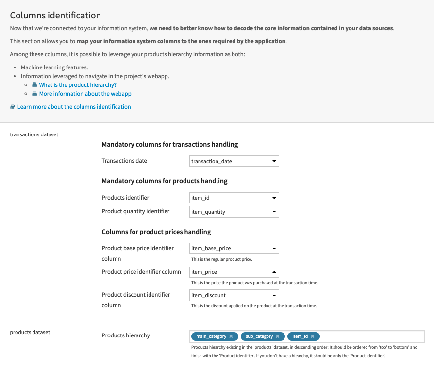
Once you’ve built all elements of the Project Setup, you can either continue to the Project View to explore the generated datasets or go straight to the dashboards and webapp to visualize the data. If you’re mainly interested in the visual components of this pre-packaged Solution, feel free to skip over the next section.

Under the hood: The Project Setup’s underlying Flow#

The Project Setup is built on top of a Dataiku Flow that has been optimized to accept input datasets and respond to your select parameters. Let’s quickly walk through the different Flow zones to get an idea of how this was done.

Flow zone	Description
inputs_zone	Contains the uploaded datasets for your distribution network (locations_dataset) and customer data (customers_dataset).
Default	Includes elements of your data that aren’t needed in the preprocessing zone (i.e data that’s already geocoded).
preprocessing_zone	Is dependent on the parameters you input to the Project Setup to define the type of your location identifiers. If input locations were defined as latitude/longitude combinations, the data is directly passed to the final prepared datasets (locations_prepared and customers_prepared). If input locations were defined as addresses, the Geocoder plugin is used to geocode the addresses. The resulting datasets are split to separate out successfully geocoded locations (locations_well_geocoded and customers_well_geocoded). These datasets are passed to the final prepared datasets. Those that couldn’t be geocoded are stored in datasets that won’t be used in the remainder of the Flow, but can be investigated to understand why they couldn’t be successfully geocoded.
isochrones_zone	Includes 3 datasets of interest created by sending each row of the locations_prepared to the selected isochrone API service to compute the requested isochrones. locations_isochrones contains, for each location, the computed isochrone areas (in geojson format), and additional information about isochrones depending on the isochrone API service used. locations_competition gives, for each location and each computed isochrone, all other locations from locations_prepared that are contained in the computed isochrone. locations_isochrones_denormalized is created to support the visualization capabilities of the Solution’s webapp by materializing and identifying the relationship between locations and their isochrones.
customers_zone	If you provided customer data to the Project Setup, this zone will: Take customers_prepared, locations_isochrones and locations_isochrones_denormalized from the previous zones to locate all customers that exist within the previously computed isochrones, as well as the distance between the location and each customer in the isochrone. Additionally, all customer information is copied over to the resulting locations_customers dataset. Finally, locations_customers_agg aggregates all customers across all isochrones for a location.
dashboards_zone	Is dedicated to the isolation of all the datasets needed to build visualizations for the two project dashboards (see below for more details).
webapp_zone	Isolates the datasets used by the Solution webapp and can largely be ignored unless you wish to make changes to the webapp. Editing these datasets will break the webapp.

Further explore your geospatial data with shareable visualizations#

The data generated by the Distribution Spatial Footprint project can be either viewed directly in the Flow in raw format, or explored through a variety of rich visualizations pre-built into dashboards.

The Locations competitors dashboard provides three charts that can be particularly useful in identifying cannibalization that’s occurring between your own points of sale, or between your points of sale and your competitors.

Within the Locations customers dashboard (if you provided customer data), you will find several pre-built charts which visualize:

The spread of customers across all computed isochrones for all locations.
A map representation of customers locations.
The number of your customers that aren’t contained in a computed isochrone.

With this information, you can optimize marketing campaigns based on customer spread, optimize your distribution network for high potential areas, and identify new store locations to draw in new customers.

Expanding analysis with an interactive webapp#

Although this Solution already contains high value visualizations in the pre-built dashboards, the geospatial analytic capabilities enable you to conduct your own visual analysis using a pre-built webapp for spatial analysis.

The webapp has several fields that you can use to impact the real-time map visualization. Please note, at this time the webapp doesn’t save your previous searches and will restore to its default empty state each time you reload it.

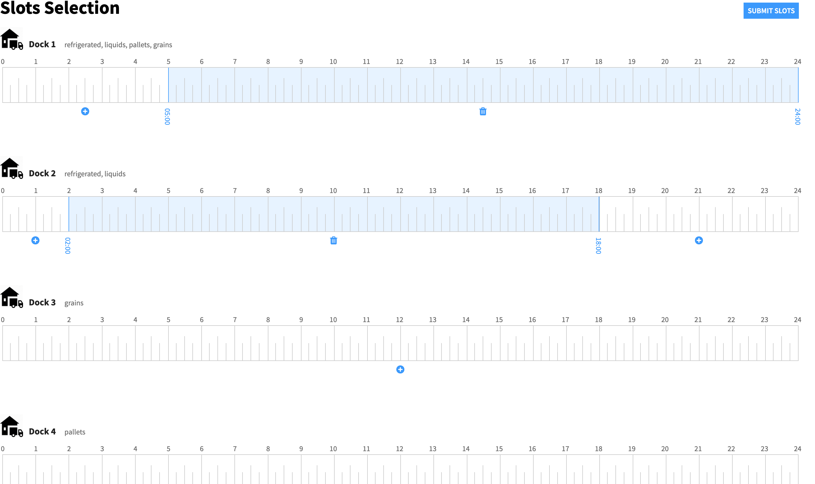
To begin, select the isochrones you would like to focus on from the full list of computed isochrones. The icon will change to reflect the transportation mode you previously selected in the Project Setup.
Within the Network Analysis section you can either individually add locations from your full list OR apply filters based on your location data (for example city, shop type, etc.).
- The number of visualized points of sale out of the total sample of Points of Sale will update with the map. You can also increase or decrease the random sample size but please be wary that larger samples might cause the webapp to slow down.
- You can display more information about a location by clicking on the location pin.
  - When displaying locations based on filter, clicking on the location pin will also allow you to deselect a specific location (that is, remove it from displaying on the map) or focus on a specific location (that is, remove all other locations from the map). This will push you into the From Location selection option. Switching back to From Filters will add all unselected locations back to the map
- Similarly, clicking on an area within an isochrone will display a card with the isochrone information
You can turn the Comparative Network Analysis section on or off by clicking the slider button. Here you can add locations for comparison using the same fields as in the network analysis section.
- Doing so has many benefits including identifying isochrone cannibalization between points of sale or identifying strategic distribution points to support all your points of sale.
- Sample size can also be independently increased/decreased here.
Lastly, if you provided customer data, you can turn on Customer Analysis with the slider button. You can’t add customers individually, but you can populate the map using filters based off of customer information in your customer dataset.
- Only customers contained in the isochrones of a location will display on the map so you must select a location.
- Customer detail will increase by zooming, and you can click on individual customer points to display the full card of customer information.
- The sample size can be independently increased/decreased, and the value you select will be a random sample of customers per location. For example, a sample size of 100 when two locations are displayed will result in 200 customers displayed on the map.

Reproducing these processes with minimal effort for your data#

The intent of this project is to enable business users to understand how Dataiku can be to conduct a spatial exploration of your distribution network.

This documentation has reviewed provided several suggestions on how to derive value from this Solution. Ultimately however, the “best” approach will depend on your specific needs and data. If you’re interested in adapting this project to the specific goals and needs of your organization, Dataiku offers roll-out and customization services on demand.