Solution | Demand Forecast

Overview

Business case

Forecasting demand accurately is critical for efficient planning—whether you’re managing inventory, staffing, production, or budgets. While many organizations still rely on manual, spreadsheet-based forecasting, these methods are often slow, error-prone, and difficult to scale.

The Demand Forecast Solution helps replace manual forecasting with a robust, automated pipeline using modern Time Series Forecasting techniques. It delivers fast and continuously updatable forecasts—designed to support both strategic “spot” planning efforts (for example seasonal campaigns or annual planning cycles) and ongoing rolling forecasts in operational environments. By implementing this Solution, you can:

• Reduce forecast errors to improve service levels and reducing safety stock.

• Save time—avoid hours of manual work each planning cycle.

• Standardize and scale your forecasting practice across teams and business units.

• Increase agility by updating forecasts monthly, weekly, or even daily as new data comes in.

Whether you’re a Planner seeking more reliable numbers, or a Data Analyst or Data Scientist looking to operationalize a modern forecasting system, this Solution provides a fast, repeatable starting point.

Installation

Dataiku 13.3+Dataiku Pre-13.3

1. From the Design homepage of a Dataiku instance connected to the internet, click + Dataiku Solutions.

2. Search for and select Demand Forecast.

3. If needed, change the folder into which the Solution will be installed, and click Install.

4. Follow the modal to either install the technical prerequisites below or request an admin to do it for you.

Note

Alternatively, download the Solution’s .zip project file, and import it to your Dataiku instance as a new project.

Technical requirements

Dataiku instance

• Have access to a Dataiku 14+* instance.

• A Python 3.10 code environment named solution_demand-forecast with the following required packages:

Jinja2>=2.11,<3.2
MarkupSafe<2.2.0
Werkzeug<3.1
cloudpickle>=1.3,<1.6
flask>=1.0,<2.3
gluonts>=0.8.1,<0.17
itsdangerous<2.1.0
lightgbm>=4.6,<4.7
mxnet>=1.8.0.post0,<1.10
numpy<1.27
pmdarima>=1.8.5,<2.1
prophet>=1.1.1,<1.2
scikit-learn>=1.0,<1.6
scikit-optimize>=0.7,<=0.10.2
scipy>=1.13,<1.14
statsmodels>=0.12.2,<0.15
xgboost>=2.1,<2.2

Warning

Make sure the pandas package version is 2.2.

Data storage

The Demand Forecast Dataiku Application is designed to work efficiently with various storage systems. It has been tested and validated on the following data connections:

• Filesystem

• Snowflake

• AWS S3

• BigQuery

• PostgreSQL

These connections support the full functionality of the application, including model training, scoring, automation, and dashboard interactivity.

Note

For any other data storage systems, usage is considered experimental and may require additional validation or customization.

Data requirements

Sales dataset

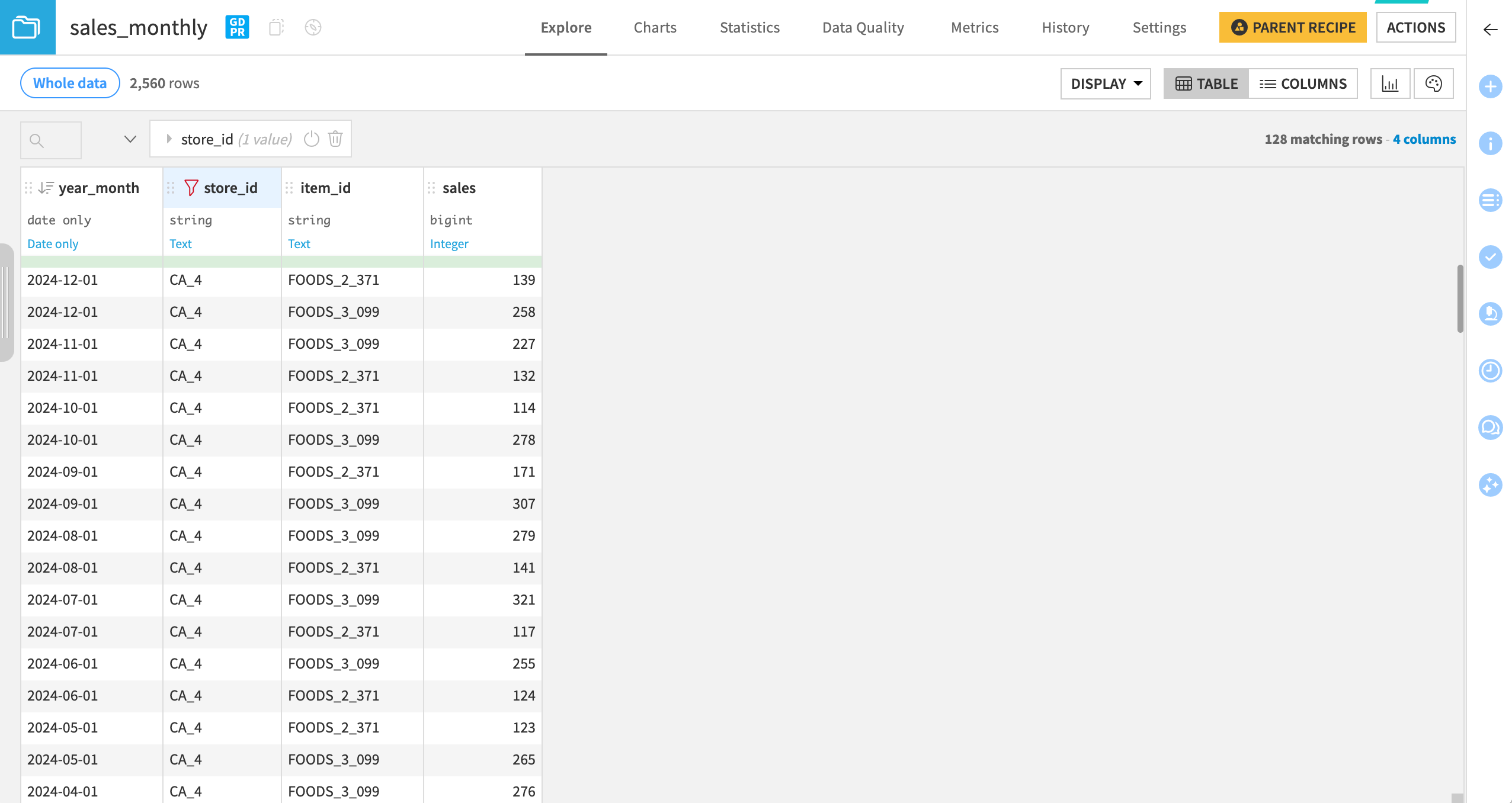
The Demand Forecast Solution requires a Sales dataset containing historical quantities sold or consumed per time step. Each value must be an integer, indexed by a timestamp and up to two Time Series Identifiers (TSIDs), for example store_id and item_id. Data must be equispaced—that is, all TSIDs must follow the same time frequency (for example daily, weekly, or monthly).

Example of Sales data:

year_month	store_id	item_id	sales
2024-11-01	CA_1	FOODS_1	100
2024-12-01	CA_1	FOODS_1	150

Pricing dataset (optional)

To account for price sensitivity and promotion effects, a Pricing dataset containing sell_price and base_price columns can be provided. Both columns are mandatory. The dataset must also cover all TSID combinations for all timestamp values found in the sales data, and for the forecast horizon.

Example of Pricing data:

year_month	store_id	item_id	sell_price	base_price
2024-11-01	CA_1	FOODS_1	1.49	1.99
2024-12-01	CA_1	FOODS_1	1.89	1.99

Legacy forecasts dataset (optional)

For benchmarking purposes, you can provide forecasts generated by your legacy forecasting system. It must contain a legacy_forecast column and align in time and segmentation with the sales data over a shared historical period.

Example of legacy forecast data:

year_month	store_id	item_id	legacy_forecast
2024-11-01	CA_1	FOODS_1	95
2024-12-01	CA_1	FOODS_1	140

Volume requirements

Time Series Forecasting (TSF) works by identifying patterns in historical data—seasonality, trends, or recurring fluctuations. To produce reliable forecasts, the underlying data must meet certain quality criteria:

• Consistent sales history

  • TSF assumes that demand has been observed regularly over time. For each combination of Time Series Identifiers (TSIDs) (for instance product_id and store_id), the sales signal must be continuous—not sporadic or irregular.

  • Sparse or highly erratic sales histories (common with slow-moving SKUs) often lack the structure needed to train meaningful forecasting models.

• Minimum history length

  • This Solution uses Dataiku’s native Time Series Forecasting engine, which enforces a minimum number of observations per time series. Cold-start products without sufficient history can’t be forecasted using this method.

• Uncapped demand

  • The model assumes that historical sales reflect true demand, not constrained by stockouts or supply limitations.

Solution scope

This Solution leverages Time Series Forecasting (TSF) and is best suited for fast-moving products with high-volume, stable, and seasonal demand. It’s not a good fit for scenarios where demand is driven primarily by external forecasts, irregular customer behavior, or sporadic consumption. We treat “demand” as historical sales or consumption volume—expressed in integers.

Good fit

• Supply Chain demand planning

  • Inventory forecasting: Anticipate future sales to optimize stock levels and avoid over/under-stocking. Works well for consumer goods, consumables, and spare parts (fast/medium movers).

  • Sourcing & production planning: Support procurement and production schedules for Make-to-Stock and hybrid models.

  • Reordering & replenishment: Predict Point of Sale needs for retail chains, pharmacies, and convenience stores.

• Workforce & capacity planning

  • Healthcare: Forecast patient flow—ER visits, lab tests, admissions.

  • Call centers: Plan staffing based on expected ticket or call volumes.

  • As long as time-based patterns exist, this is a strong fit.

• Marketing & promotion optimization

  • Quantify baseline demand to assess uplift from campaigns or schedule promotions for peak/low periods. Particularly relevant in CPG, e-commerce, telco, and media.

  • Combine the Demand Forecast Solution with the Solution | Markdown Optimization for automated pricing and promotion insights.

• Financial planning: see “Revenue forecasting” section below.

Not a fit

• Slow-moving products: When demand is sporadic or driven by a few large clients.

• Make-to-order or custom manufacturing: Forecasting demand for one-off, capital-intensive items isn’t viable.

Revenue forecasting: The right Solution

You can approach revenue forecasting in two main ways:

1. Bottom-up approach: This method predicts the quantity of “product” sold at a granular level (for example, units per product or category) and multiplies by price to estimate revenue. Forecasts are based on prior sales data and drivers at the same or higher granularity, such as weather, holidays, or customer/product attributes. If this describes your use case, then you can use this Demand Forecast Solution.

2. Top-down approach: This method forecasts total revenue directly for a business unit, without using unit sales * price as an intermediary. Forecasts are based on historical revenue figures and numerical drivers relevant to revenue streams. If this describes your usage, then you should use the Solution | Financial Forecasting instead.

Each approach lends itself more readily to different industries and expectations. Top-down approaches are most often seen when firms are selling bundles of products, or generating streams of revenue, such that counting individual products with consistent specific prices isn’t well matched to their business reality.

Workflow overview

• Configure and run the Solution

• Review forecasts with planners in the Demand Explorer dashboard

• Inspect or refine the model in Visual Analysis

• Automate retraining and forecast delivery with Scenarios

• Monitor forecast impact on operations

Note

You can follow along with the Solution in the Dataiku gallery.

Walkthrough

Context

Let’s take the example of a retailer running biannual planning cycles (June and December) to prepare for major demand periods like back-to-school and the holidays. They forecast demand monthly, six months ahead, to inform procurement, production, and marketing. These forecasts are typically broken down by product, location, or channel.

Challenges:

• Manual forecasts were inaccurate and labor-intensive.

• Safety stock levels needed to be kept high, leading to excessive inventory holding costs, costly last-minute orders, and missed supplier discounts.

Goal:

• Improve forecast accuracy and reduce manual effort by:

  • Using machine learning and time series modeling techniques that integrate historical sales data and capture seasonality and trend.

  • Automating the forecast pipeline process (data ingestion, model training, and forecast generation).

Configuring the Solution

For this hands-on walkthrough we use a selection of real-world data from Walmart (via the Kaggle “M5 Forecasting Accuracy” Challenge), aggregated monthly.

Step-by-step:

1. Load the data into a prep project in Dataiku. Here, we only need to parse dates in the year_month column.

2. Install the Demand forecast Solution. This creates a new project.

3. Open the Solution project and click the Project setup button on the project’s home page.

4. Under Input datasets, select your prep project and the according prepared sales dataset.

5. On the Column mapping section:

• Map the Sales column to sales.

• Map the Time Series identifer columns to store_id and item_id.

• Confirm that Timestamp and Time step are auto-detected as year_month and monthly respectively.

6. Set the forecast horizon to 6 months.

7. Keep the default performance metric and click Run Now.

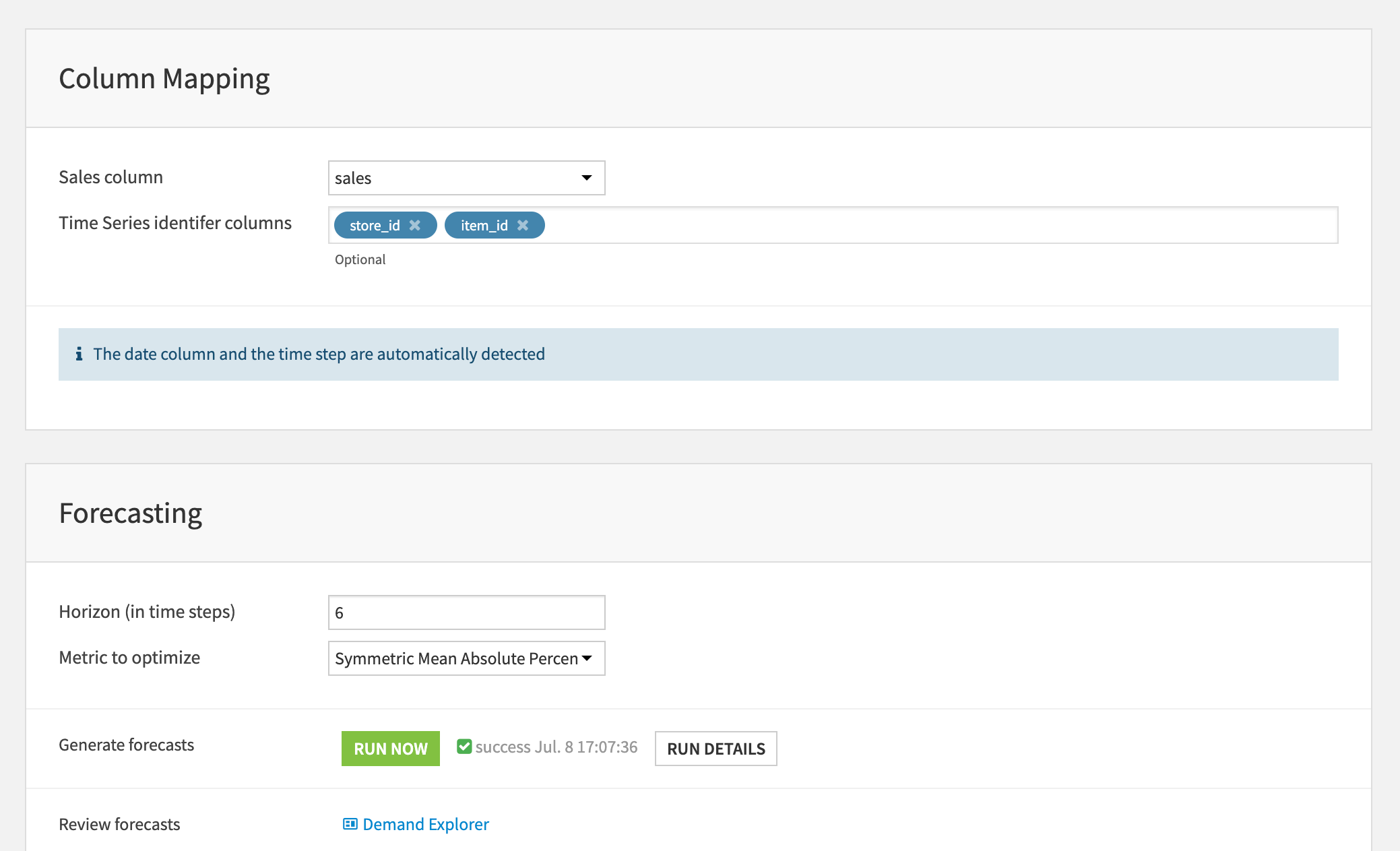
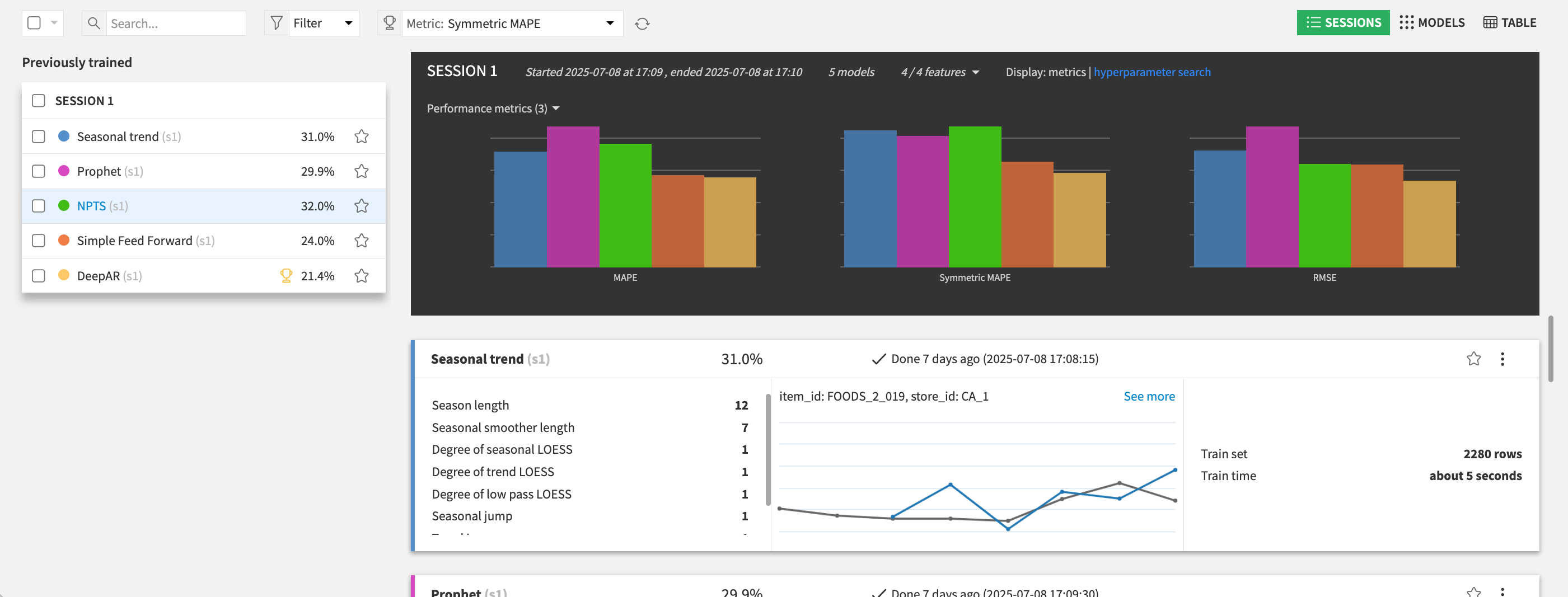
Behind the scenes:

• The Solution evaluates multiple forecasting algorithms (from classical statistical methods to modern ones such as Prophet and Deep Learning).

• It uses part of the history as a holdout (backtest) to assess accuracy.

• Forecasts are generated for both the backtest period and future horizon.

Solution deliverables

When the run is over, click on Demand Explorer to review forecasts.

This pre-built interactive dashboard helps business users validate demand forecasts before making decisions. It compares actual sales, model-generated forecasts, and optional legacy forecasts over time, using an intuitive chart and a pivot table. Users can filter by product, store, or any business dimension to inspect forecast accuracy across combinations, time steps, or aggregated totals. It supports both backtest validation and forward-looking sanity checks, ensuring forecasts are reliable for planning activities such as inventory, procurement, or staffing.

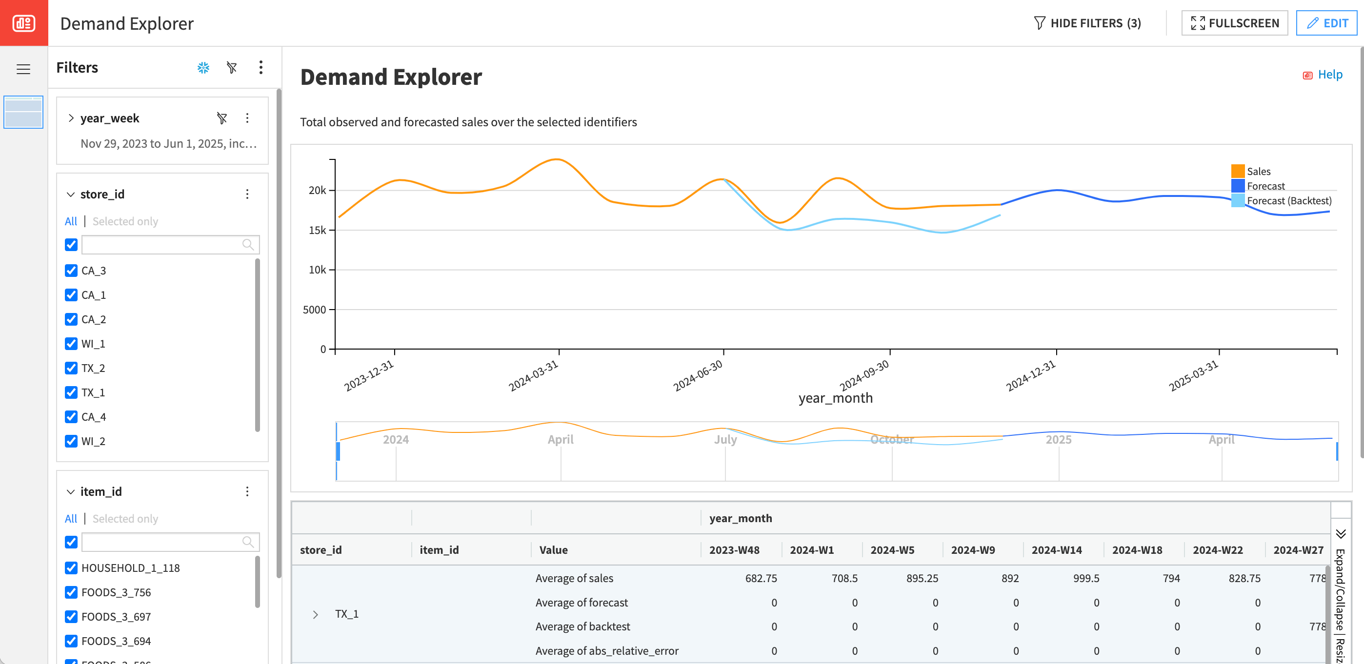
Individual forecast values are also available in a dataset in the project Flow. They’re generated by a Scoring recipe, which uses a forecasting model as input.

To inspect or refine the model:

• Open the Visual Analysis environment.

• Review algorithm choice and settings.

• Rerun or compare models as needed.

• Open model views to further inspect them.

Going further

Improving operations with ongoing rolling forecasts

Every month, our retailer’s supply chain team must determine how much inventory to stock at each central distribution center and individual store to meet customer demand. Historically, they used a fixed replenishment model: each store placed one order per month, with the goal of maintaining a 34-day Inventory Coverage Level (ICL) to avoid stockouts.

This strategy had major drawbacks. Inaccurate forecasts led to excessive safety stock and high inventory carrying costs. Analysis showed that a 10% reduction in MAPE would lower ICL by 4 days—translating into millions of dollars in annual savings at central warehouses alone.

To unlock this value, the model must be retrained and new forecasts regenerated monthly, as fresh sales and context data become available. The Demand Forecast Solution can support this workflow and can be adapted for automated retraining and forecast delivery, as explained in the Solution Wiki.

Improving accuracy with exogenous variables

Beyond historical sales, forecasts can be improved by incorporating external signals such as:

• Weather

• Holidays and promotional calendars

• Regional consumption patterns

• Local events

• Economic indicators (for example population growth and inflation)

Dataiku’s powerful data prep and Visual Time Series capabilities make it easy to ingest, clean, and join these variables—enabling models to capture complex or shifting demand patterns.

Monitoring the impact of forecasting

Improved forecasts alone aren’t enough—you must also monitor how forecasts drive operational decisions.

In inventory planning, this means verifying that cost reductions don’t come at the expense of service levels. Beyond MAPE, we would recommend tracking:

• Forecast Bias (to detect systemic over/under-forecasting)

• Service Level Metrics (for example, % of orders fulfilled on time)

• Fill Rate (actual demand met vs. forecasted)

Tracking these metrics helps ensure that inventory reductions are the result of smarter forecasting—not lower product availability.

These KPIs can be monitored in your existing BI platform or directly within Dataiku using Dashboards and Scenario Reporting.

Reproducing with minimal effort for your data

The primary goal of this Solution is to help Planners benefit from modern forecasting techniques that improve accuracy compared to traditional spreadsheet-based tools—and to accelerate delivery for Data Analysts and Data Scientists responsible for building and operationalizing forecasts.

While the walkthrough focused on a Retail use case, the Solution is flexible and can be applied to transform operations across many industries, including:

• Manufacturing and supply chain

• Healthcare and workforce planning

• Telecommunications and utilities

• B2B and wholesale distribution

You can easily adapt the Solution to your own context by changing a few settings. Common variations include:

• Time Granularity: Switch from monthly to weekly data for faster planning cycles or more reactive operations.

• Forecast Horizon: Adjust the length of the forecast window to reflect your planning needs (for instance, 2 weeks vs. 12 months).

• Forecast Scope: Instead of store_id, you can segment forecasts by:

  • Sales channel (for example, online vs in-store)

  • Region (for example country, warehouse zone)

  • Customer (in B2B contexts)

• Single TSID Models: If you want to forecast:

  • Per product (across all locations or customers)

  • Per scope (for example, all items sold in a given store)

  • In the prep project, simply add a Group recipe to sum sales per time step and one of the TSIDs. Provide its output dataset as input to the Solution.

Test configurations in parallel by duplicating an existing Demand Forecast project or installing fresh copies from the Dataiku Solutions Store.

This documentation has provided several suggestions on how to derive value from this Solution. Ultimately however, the “best” approach will depend on your specific needs and data. If you’re interested in adapting this project to the specific goals and needs of your organization, Dataiku offers roll-out and customization services on demand.