Solution | Credit Risk Stress Testing (CECL, IFRS9)#

Overview#

Business case#

Precise modeling of credit loss is a critical regulatory activity for all financial institutions. It requires efficient forecasting for each credit portfolio, rapid aggregation and analysis of the overall impact on the company balance sheet, and guaranteed end-to-end governance.

While being a well established exercise, this work can consume large amounts of effort from risk and finance teams, and often runs on a patchwork of systems with outmoded architectures. Whether for regular or ad hoc reviews, this process requires processing of large and varied datasets through complex transformations and iterative modeling steps to obtain robust final figures. The challenges facing this work are well understood, with pressure only growing: risk managers highlight legacy IT systems (86%) and a lack of accessible, high quality data (63%) as core challenges in prior years. Teams face a clear decision point between doubling down on investments in legacy systems, or reorienting to a modernized risk management estate.

Dataiku’s Credit Risk Stress Testing solution supports standardized credit risk portfolio modeling exercises (including CECL & IFRS9) and ad hoc credit stress testing analyses. It offers risk and finance teams an opportunity to confidently transition to a modernized data pipeline and modeling approach, delivering improved efficiency and flexibility alongside full governance and auditability. With only a few steps, you can scale the solution across credit portfolios to create comprehensive complete credit exposure modeling with extensive governance.

Installation#

The process to install this Solution differs depending on whether you are using Dataiku Cloud or a self-managed instance.

Dataiku Cloud users should follow the instructions for installing solutions on cloud.

The Cloud Launchpad will automatically meet the technical requirements listed below, and add the Solution to your Dataiku instance.
Once the Solution has been added to your space, move ahead to Data requirements.

Technical requirements#

To leverage this Solution, you must meet the following requirements:

Have access to a Dataiku 12.0+* instance.
Install the Time Series Preparation Plugin (if not yet installed).
A Python code environment named solution_credit-stress-testing with the following required packages:

kaleido==0.2.1
plotly==5.14.1
scipy==1.7.3

Data requirements#

The project is initially shipped with all datasets using the filesystem connection.

The mortgage data comes from Freddie Mac. The project requires the historical performance of the loans to understand how economic conditions affected them.
Economic Data both for history and forecast come from The Federal Reserve.
Housing Price Indices by State come from the Federal Housing Finance Agency.

The Solution needs this exhaustive historical data to build the models. However, when running the ECL computation, historical data is no longer needed. The Solution applies the models to the most recent snapshot against the economic scenarios.

Workflow overview#

You can follow along with the Solution in the Dataiku gallery.

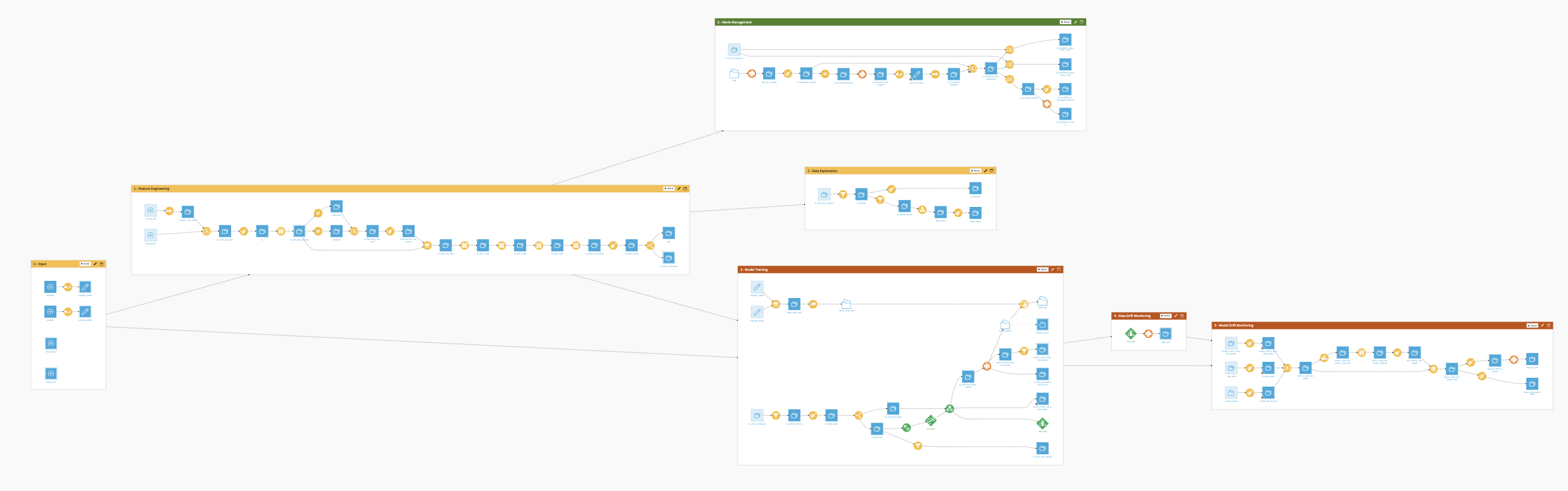
The project has the following high-level steps:

Build probability of default and loss given default models using both visual and code tools.
Explore your models with pre-built visualizations.
Industrialize the expected credit losses runs through the Project Setup.

Walkthrough#

Note

In addition to reading this document, it’s recommended to read the wiki of the project before beginning to get a deeper technical understanding of how this Solution was created and more detailed explanations of Solution-specific vocabulary.

Gather input data and prepare for training#

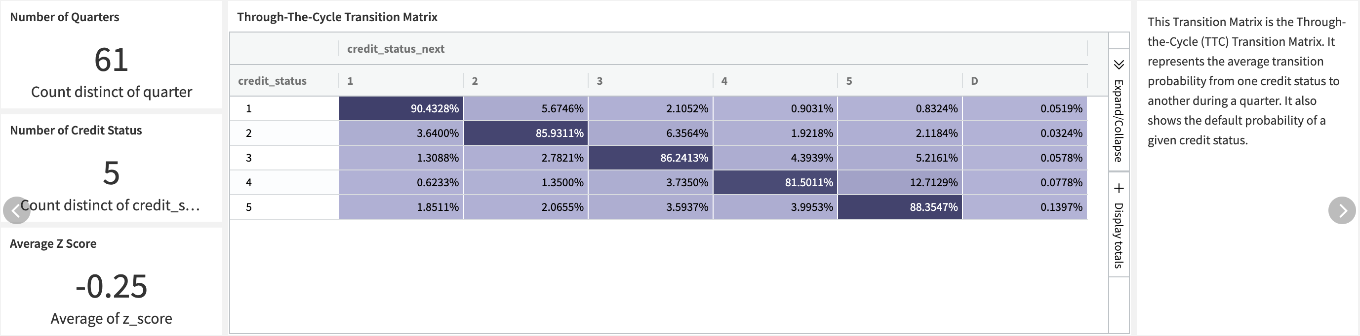
Both the Through-the-Cycle (TTC) matrix and the Point-in-Time (PIT) matrices are built using visual recipes along with the $`x`$ density coordinates of each bin, to compute the z-score afterward.

A Window recipe computes for each loan the credit status for the next period.
Two Group recipes will compute the matrices:
- One Group recipe takes care of the TTC matrix by aggregating using credit status and next credit status as keys.
- The other handles the PIT by adding the quarter as a key.
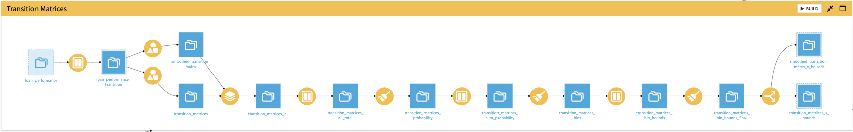
The project stacks two sets of matrices back together and then goes through a series of visual recipes to compute the probabilities of transitions and their equivalent as $`x`$ density coordinates:
- The total UPB is computed for each transition starting point, the key being quarter and credit status.
- The probability is computed as the ratio between the transition UPB and the total UPB.
- For each transition starting point the cumulative probability is computed.
- Cumulative probabilities are converted into the normal density.
- The previous bin is retrieved for each row.
- Finally, the initial normal density coordinate is set to -Infinity for each transition starting point.
The two types of transition matrices are split back.

In parallel, the project prepared macroeconomic data to be joined with the credit data and build the probability of default model.

The macroeconomic indicators are the economic time series that relate to the credit cycle. The probability of default model will use some of these variables as predictors.

The economic data also comes with forecast scenarios. They might follow a baseline scenario and a more adverse one like in this example. It’s reflected at different levels depending on the variable.

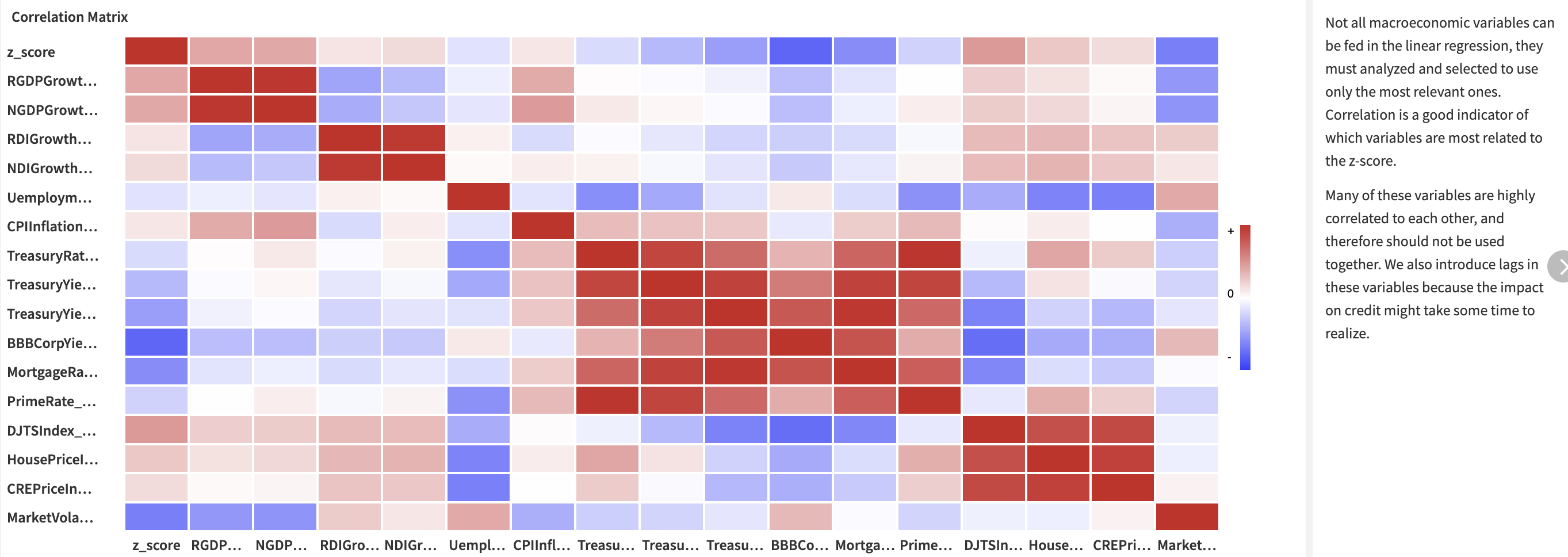
The project includes a correlation matrix built using a statistics card. It provides a fast and visual way to identify the groups of variables closely correlated to each other. Eventually, it delivers a first view on the variables that are more likely to predict the credit variable z-score. You will add lags on each of the economic variables to find the right delay between the economic observation and the actual credit consequence.

Building a probability of default model using z-score modeling#

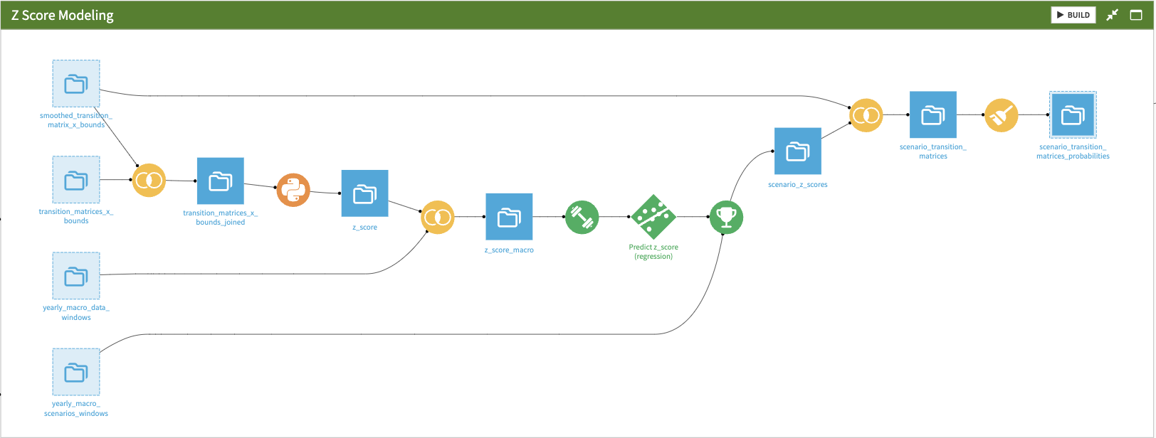
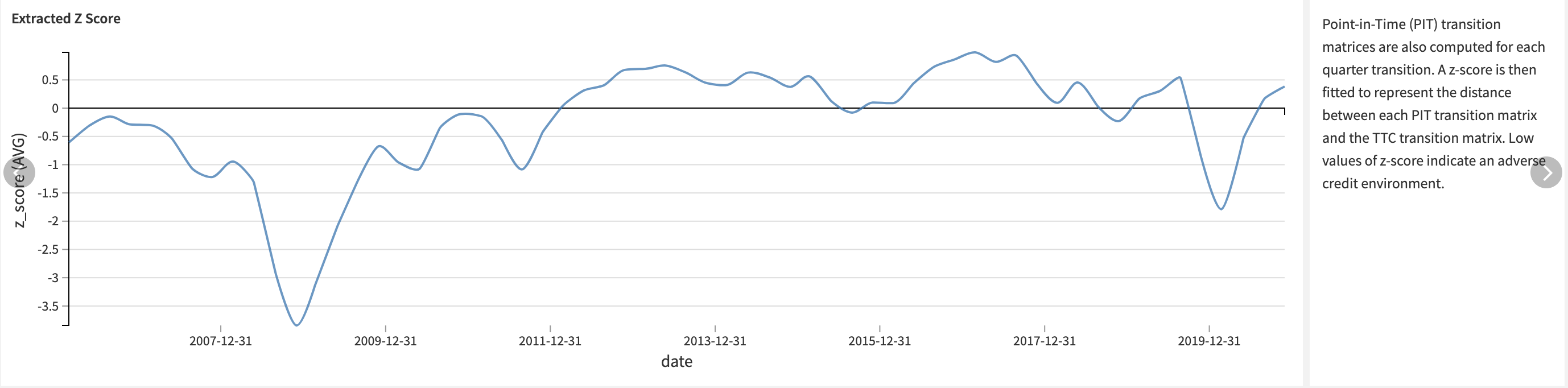
The project builds the z-score from the transition matrices, trains a linear model on the macroeconomic data, and scores forecasts against this model.

First, the project joins the TTC transition matrix dataset to the PIT transition matrices datasets. This will be the input of the z-score extraction.

The Solution achieves z-score extraction in the Python recipe:

The objective function for each quarter is defined. This is what $z$ optimizes.
The global objective function on $z$ variance is defined. This is what $\rho$ optimizes.
First $\rho$ is optimized and saved as a project variable.
Then using this value, $z$ is optimized and saved in the output dataset.

The Solution joins the extracted Z-score to the prepared macroeconomic data to create the input of the linear regression model that’s handled using the visual ML module.

The project looks to fit an ordinary linear regression to predict the z-score, using some macroeconomic variables or their lags that have been previously prepared. To select the variables, the project iterates on the feature reduction methods to find the top three variables that are most often relevant. This example ended up using these three variables:

The BBB Corporate Yield lagged twice.
The Mortgage Interest Rate lagged three times.
The Market Volatility Index lagged once.

You can adapt this selection based on the user’s expertise or the need for the model to be sensitive to some specific features, like inflation. These three features are selected in the feature handling and the final model run using them, without any additional feature reduction.

The trained model then scores the forecasts and obtains the predicted Z scores. They’re joined to the TTC transition matrix to construct the predicted forecast matrices built in the final Prepare recipe.

Modeling loss given default using peak-to-trough#

The peak-to-trough modeling approach for loss given default (LGD) represents a conservative strategy that delves into historical worst-case scenarios for asset value declines. This method involves calculating the most significant difference between consecutive peaks and troughs in asset values. This approach is particularly pertinent as defaults often tend to spike during these trough periods.

You can perform these calculations on multiple levels, including geographical and asset class considerations. For instance, in the context of mortgages, assets can be further categorized into various subgroups like houses and flats, urban and rural properties, etc.

This project focuses on housing prices at the state level in the United States. It reveals significant variations in peak-to-trough ratios among different states, as illustrated in the graph below.

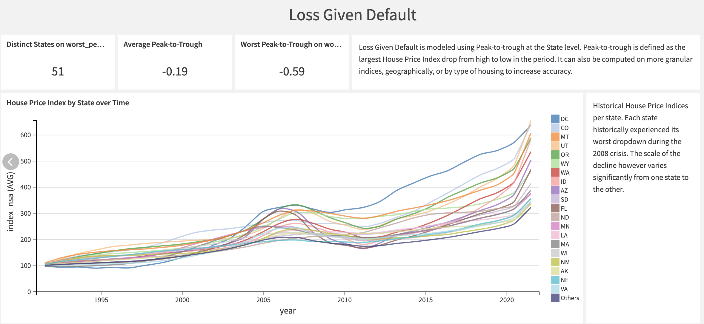
House price indices are available for all states. Upon examination, it becomes evident that certain time series exhibit more significant fluctuations compared to others. States with more pronounced peak-to-trough variations are generally considered to be riskier in terms of housing market stability.

Industrialize your ECL process through a Project Setup#

The project setup lets a user from a monitoring or execution team perform the needed ECL runs. Have approved and delivered models, you can apply them to compute ECL through a no-code interface similar to the one designed here.

The ECL Run section lets the user select the cut-off date, the ID of the PD model and the scenarios to run.

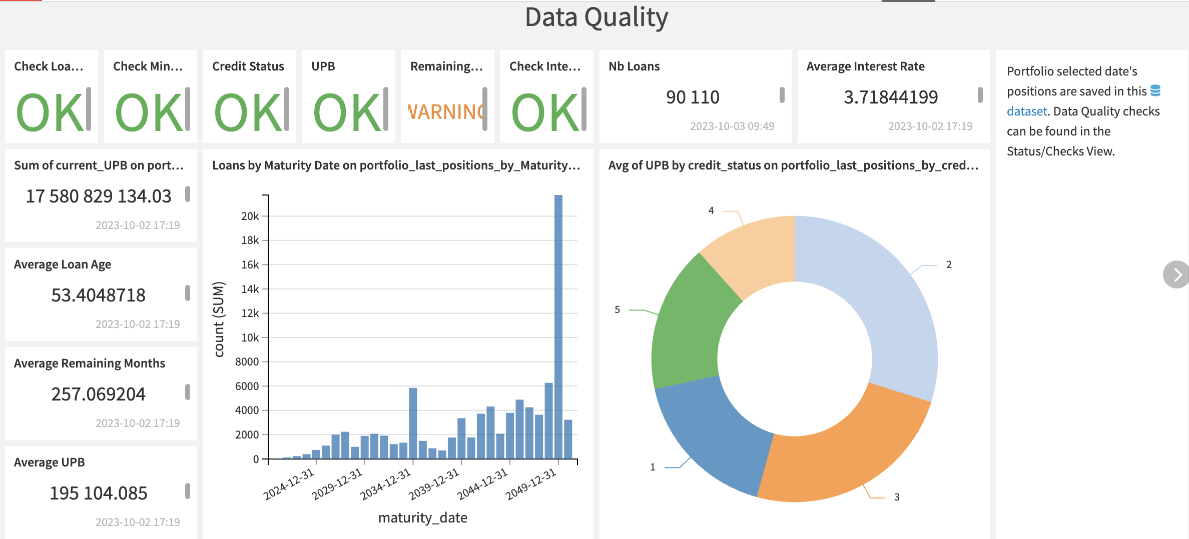
A dashboard that provides information about the data quality checks and the ECL results summarizes the output.

The second section contains an interface to select a starting and closing configuration between each a waterfall chart will be built. The [Compute Waterfall](scenario:COMPUTEWATERFALL) scenario will sequentially call the Run Simulation scenario for each needed configuration and results will be compiled in the [waterfall](dataset:waterfall) dataset.

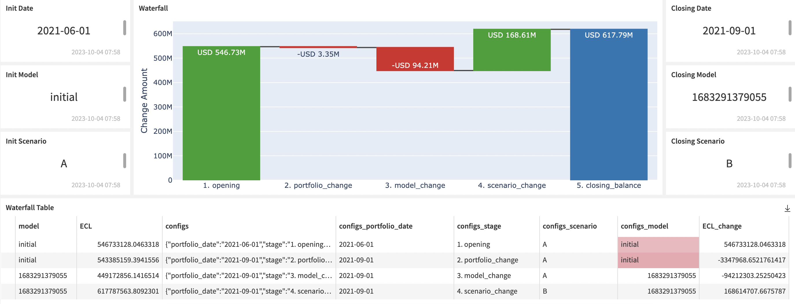
The start configuration is displayed on the left while the closing configuration is on the right.

Both configurations must define a portfolio date, a model and a scenario. Hence, the waterfall chart will compare the two final ECL values through these three potential variations: portfolio, model, and scenario.

Reproducing these processes with minimal effort for your data#

The intent of this project is to enable risk and finance teams to understand how they can use Dataiku to confidently transition to a modernized data pipeline and modeling approach.

By creating a solution that can be scaled across credit portfolios with just a few steps, you can create comprehensive and complete credit exposure modeling with extensive governance.

This documentation has reviewed provided several suggestions on how to derive value from this Solution. Ultimately however, the “best” approach will depend on your specific needs and data. If you’re interested in adapting this project to the specific goals and needs of your organization, Dataiku offers roll-out and customization services on demand.