Solution | Insurance Claims Modeling

Overview

Business case

Generalized linear models (GLMs) are a common approach to consumer insurance claims modeling across the world, with a deep, rich, and proven track record. They’re an industry standard, well-understood, and acceptable to stakeholders inside and outside the insurance firm.

Existing no and low code platforms for building and approving GLMs are often outdated and lack modern data science and analytic capabilities. They require complex and potentially unreliable nests of supporting systems to work effectively.

This Solution acts as a template of how actuaries could use Dataiku to perform their work. By using this Solution, actuaries can benefit from training GLMs in a visual environment, conduct extensive exploratory data analysis, and push their models to production through an API deployment interface.

Technical requirements

To use this Solution, you must meet the following requirements:

• Have access to a Dataiku 14.3+* instance.

• Generalized Linear Models plugin version 2.0.2+.

• A Python 3.10 code environment with pandas=1.3 named solution_claim-modeling with the following required packages:

MarkupSafe<2.2.0
Jinja2>=2.11,<3.2
cloudpickle>=1.3,<1.6
flask>=1.0,<2.3
itsdangerous<2.1.0
lightgbm>=4.6,<4.7
scikit-optimize>=0.7,<=0.10.2
statsmodels>=0.12.2,<0.15
Werkzeug<3.1
xgboost>=2.1,<2.2
gluonts[torch]>=0.8.1,<0.17
pmdarima>=1.2.1,<2.1
prophet>=1.1.1,<1.2
numpy<1.27
mxnet>=1.8.0.post0,<1.10 # Mxnet is deprecated. It will be retired in the next major DSS version.
torch>=2,<2.8
--extra-index-url https://download.pytorch.org/whl/cpu
glum==2.6.0
scipy>=1.13,<1.14
scikit-learn==1.3.2
dash==2.3.1
dash_bootstrap_components==1.0

Data requirements

This walkthrough now starts from a single synthetic input dataset that encodes assumptions about target distributions and how drivers and vehicles relate to claim behavior. The dataset contains 1,000,000 rows that simulate one year of activity for a portfolio of policyholders, and every row is keyed by a unique policy_id.

The target and exposure variables are:

• exposure—contract duration in years.

• claim_count—number of claims observed during the period.

• total_claim_amount—cumulative claim amount for the period (empty when there are no claims).

Driver-focused explanatory variables include:

• driver_age

• gender

• driving_license_age

• bonus_malus_level

• region

• annual_mileage_km

Vehicle-focused explanatory variables include:

• vehicle_age

• vehicle_power_hp

• vehicle_brand

• fuel_type

• vehicle_parking

Workflow overview

You can follow along with the Solution in the Dataiku gallery.

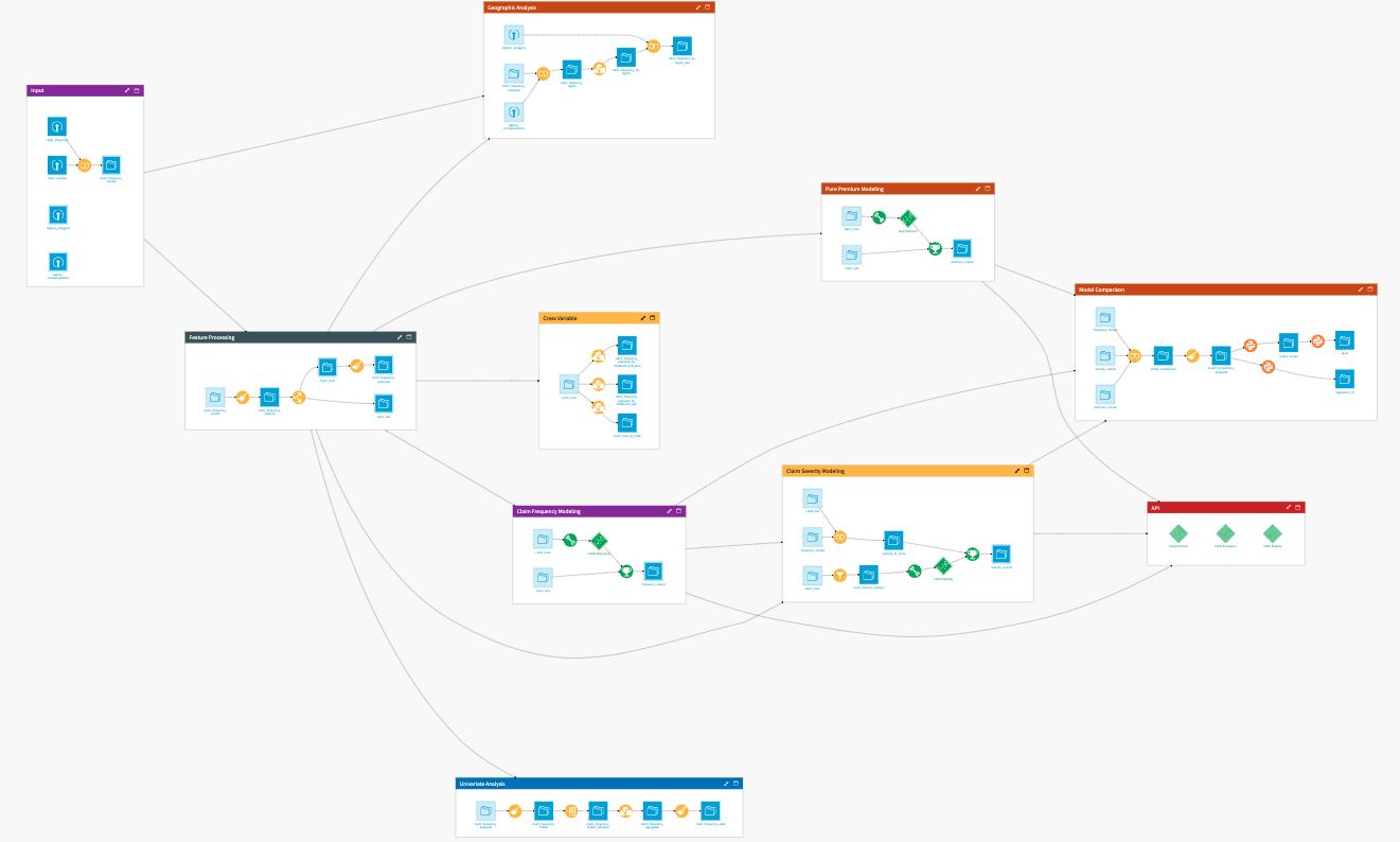
The project has the following high-level steps:

1. Input historical data and perform feature processing.

2. Conduct exploratory data analysis for a deeper understanding.

3. Train models for claims modeling and pricing.

4. Review model performance.

5. Deploy models to an API for real-time predictions.

6. Interactively explore the models’ predictions with a pre-built webapp and dashboard.

Walkthrough

Note

In addition to reading this document, it’s recommended to read the wiki of the project before beginning to get a deeper technical understanding of how this Solution was created and more detailed explanations of Solution-specific vocabulary.

Gather input data and prepare for training

The Input Flow zone ingests a single synthetic dataset (15 columns, 1,000,000 rows) that already reflects policy-level features, exposures, claim counts, and total claim amounts. That dataset feeds the Feature Processing zone, where an initial Prepare recipe caps exposure at 1 (one year of coverage), limits claim_count to 4, fills missing total_claim_amount values with 0, and labels empty vehicle_parking entries as Street for conservative modeling.

From there, a regression splines plugin recipe transforms driver_age into three basis functions with knots at 25 and 50 and a degree of 1 so that the sharp changes observed in frequency can be encoded without losing transparency. The dataset is then split deterministically into claims_train (about 91%) and claims_test via a modulo operation on policy_id to keep splits reproducible.

Additional feature engineering recipes—still within Feature Processing—standardize aggregations and prepare long-format analytical datasets for the dashboards and model training zones discussed below. With those assets in place, the workflow pivots to exploratory analysis before touching the visual ML steps.

Extensive exploratory data analysis for a deeper understanding

Two Flow zones concentrate the exploratory workload and keep insights reproducible:

Flow zone	Description
Univariate Analysis	Transforms the training set into a long format, computes weighted statistics, variances, and confidence intervals, then unfolds results for every feature.
Overall Stats	Aggregates key KPIs (exposure, claim counts, total claim amounts) so analysts can benchmark frequency, severity, and pure premium before modeling.

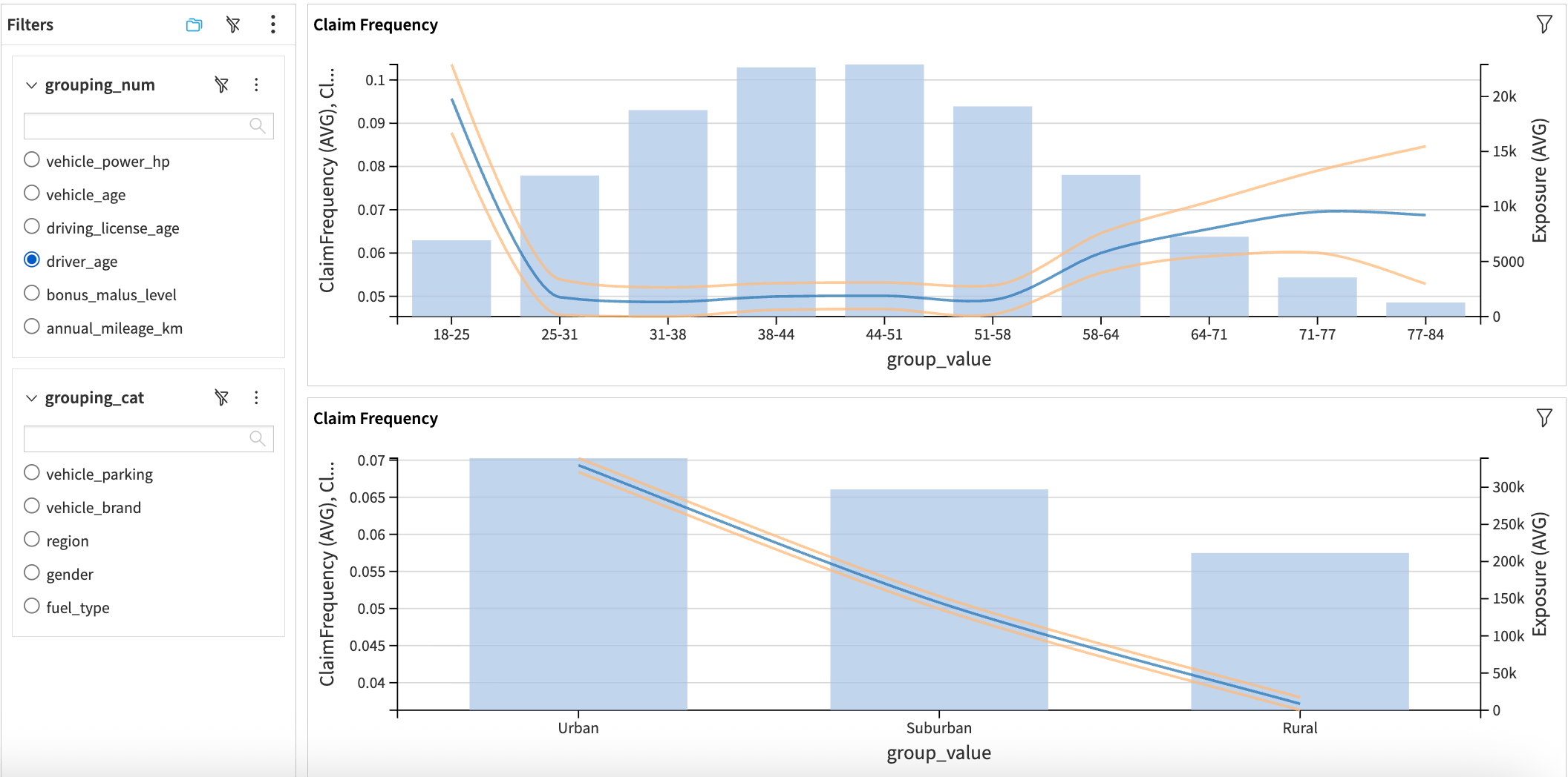
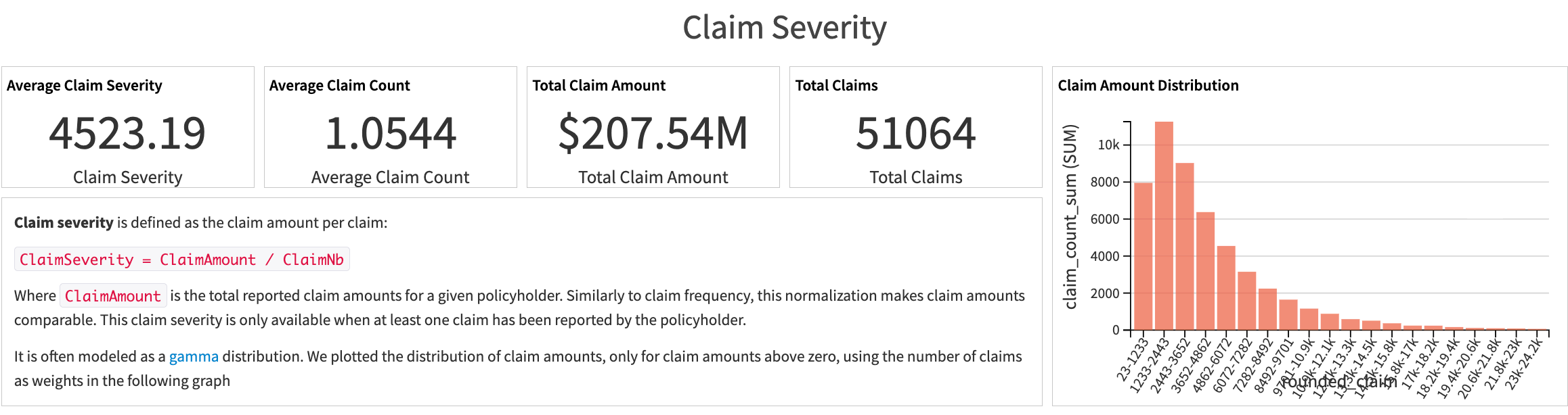
Within Univariate Analysis, claims_train is rounded (for example, mileage buckets), folded, and enriched with weights. Subsequent recipes calculate variances for claim frequency, severity, and pure premium, then aggregate by grouping attribute before unfolding the data again. The process yields long-form tables that power the Claim Frequency, Claim Severity, and Pure Premium dashboard tabs, each complete with 95% confidence bands for both numeric and categorical variables.

The Overall Stats zone complements those charts by summarizing exposure and claim distributions, including datasets such as pure_premium_total, total_claims, claim_severity_total, and claim_frequency_total. Reviewing these KPIs upfront clarifies how the synthetic portfolio behaves before moving on to the Visual GLM steps.

Train models to predict claim frequency, severity, and amount

Three dedicated Flow zones orchestrate the Visual GLM experience (one per target). Each starts from curated datasets and leverages the GLM plugin’s visual interface for configuration, diagnostics, and deployment:

Flow zone	Description
Claim Frequency Modeling	Predicts the count of claims per policyholder using a Poisson GLM with a log link and the exposure column as offset.
Claim Severity Modeling	Focuses on claim amounts for rows where claims exist (ClaimNb > 0) and uses a gamma distribution with a log link.
Pure Premium Modeling	Directly models claim amount per exposure via a Tweedie distribution (variance power 1.5) without filtering out zero-claim rows.

The model building happens in the visual GLM. The walkthrough below illustrates the claim frequency build, which then serves as the template for severity and pure premium experiments.

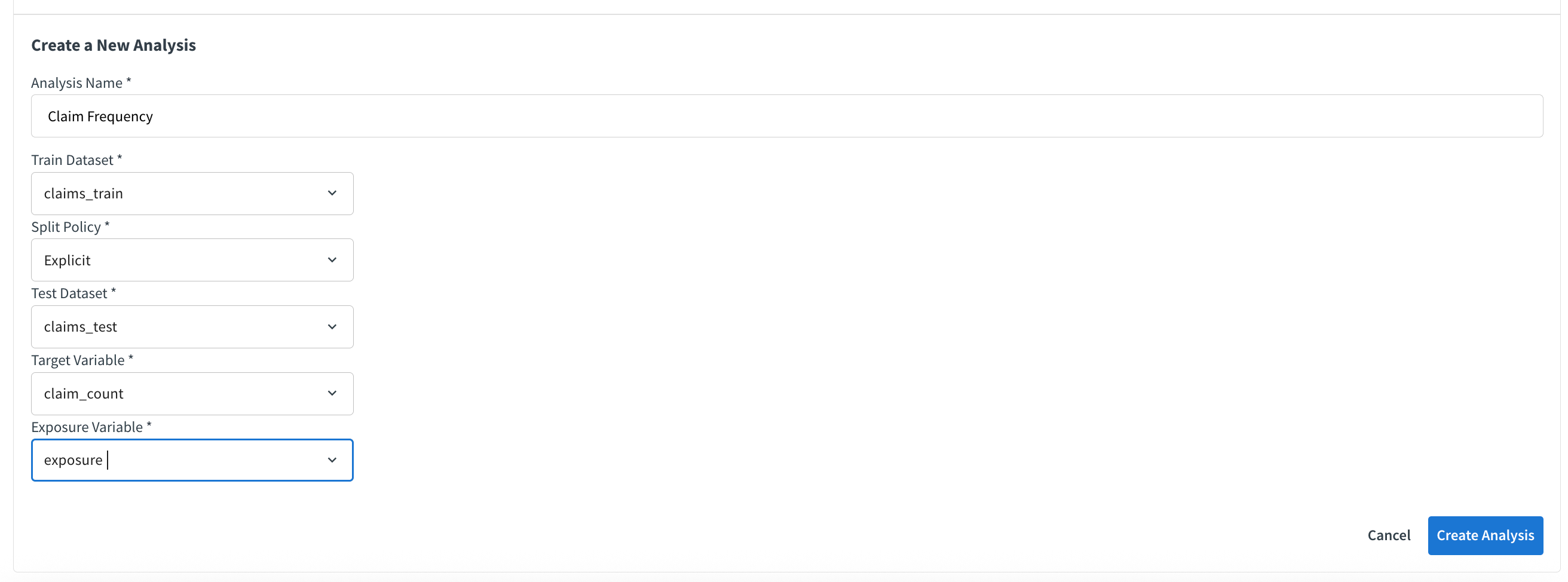
Create the analysis. From the model list, choose Or create a new analysis… and populate the wizard with: Analysis Name (Claim Frequency), Train Dataset (claims_train), Split Policy set to Explicit, Test Dataset (claims_test), Target Variable (claim_count), and Exposure (exposure). This establishes paired train/test datasets so downstream diagnostics remain aligned with the rest of the Flow.

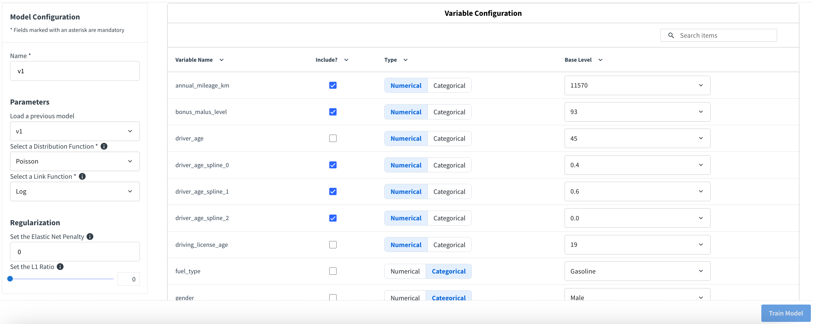
Configure the GLM. On the configuration screen select:

• Distribution Function: Poisson

• Link Function: Log

• Elastic Net Penalty: 0

• L1 Ratio: 0

Leaving the penalties at zero lets actuaries inspect un-regularized coefficients first, with the option to revisit shrinkage if non-significant terms emerge. At this stage we curate the feature list based on earlier EDA, ensure the spline features derived from driver_age share coherent base levels, and adjust categorical references away from the default “highest exposure” rule when business context suggests better anchors.

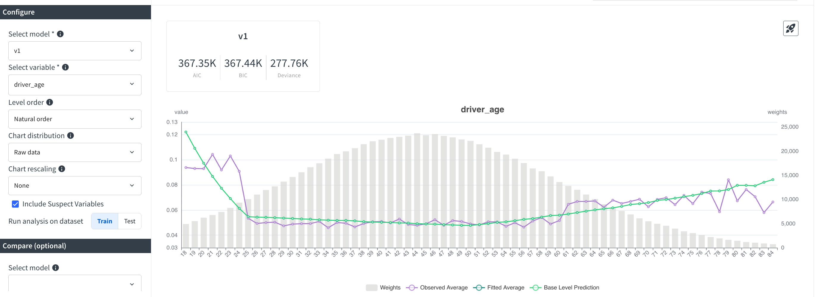
Train and inspect. After naming the model, trigger training and open the Predicted vs. Observed Chart tab. Plotting the spline expansion of driver_age confirms the sharp dip for younger drivers is now captured smoothly; residual gaps appear mainly before age 25, signaling optional follow-up feature work.

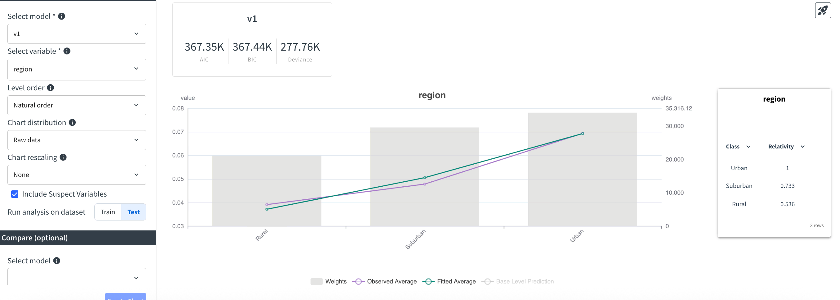
Switching the same chart to region—especially on the test sample—shows the model honoring stark relativities (for example, Rural exposure landing near 0.537 of the Urban baseline) without destabilizing between splits.

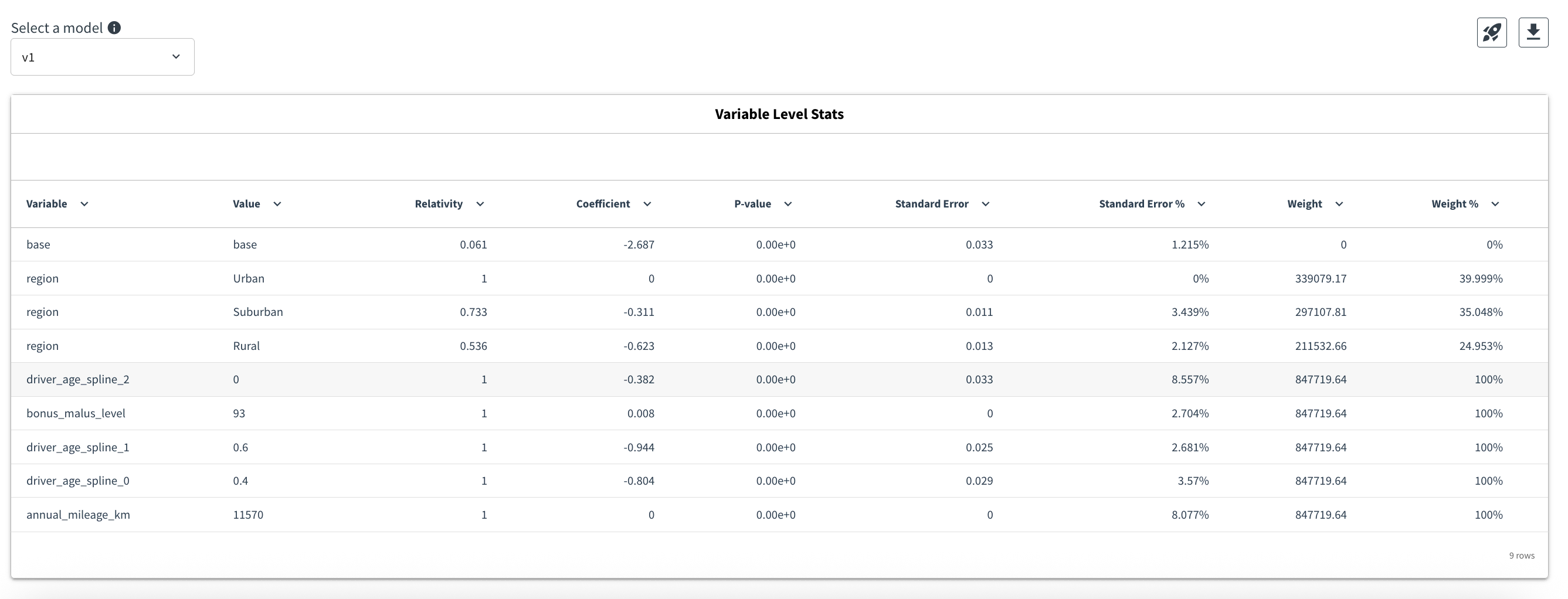
Validate coefficients. The Variable Level Statistics tab reports p-values rounded to zero and low standard deviations for this run, indicating robust coefficient significance. If a future iteration surfaces weaker signals, this is where experimenting with non-zero Elastic Net settings becomes useful.

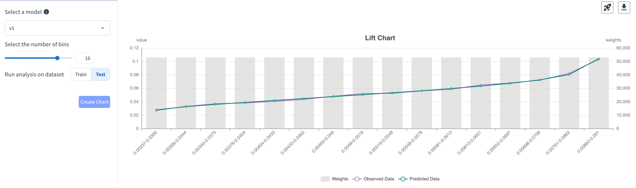
Check lift and finalize. The Lift Chart tab slices predictions into up to 16 bins (using the test data in our review) and shows a balanced fit without pronounced outliers, reinforcing deployment readiness.

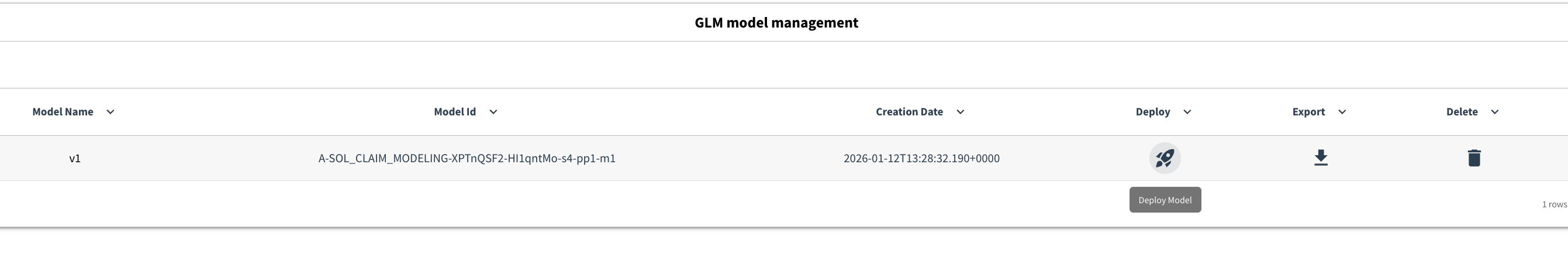
On the final tab you can deploy, delete, or export the trained object, and you can jump back into the visual ML session for deeper inspection. For this Solution we deploy the artifact so it can power both batch scoring and the downstream API use cases.

Very similar steps produce the first-pass models for claim severity (Gamma distribution with Log link and ClaimNb > 0 filtering) and pure premium (Tweedie distribution with variance power 1.5, Log link, and exposure as weight), each time leveraging the insights gathered during EDA to decide feature inclusion and base levels.

Evaluate model performance

The Model Comparison Flow zone consolidates the scored holdout datasets from each modeling zone and joins them on their shared policy_id. A Prepare recipe computes the Compound Model prediction by multiplying claim frequency and severity scores so it can be contrasted with the Tweedie (pure premium) prediction.

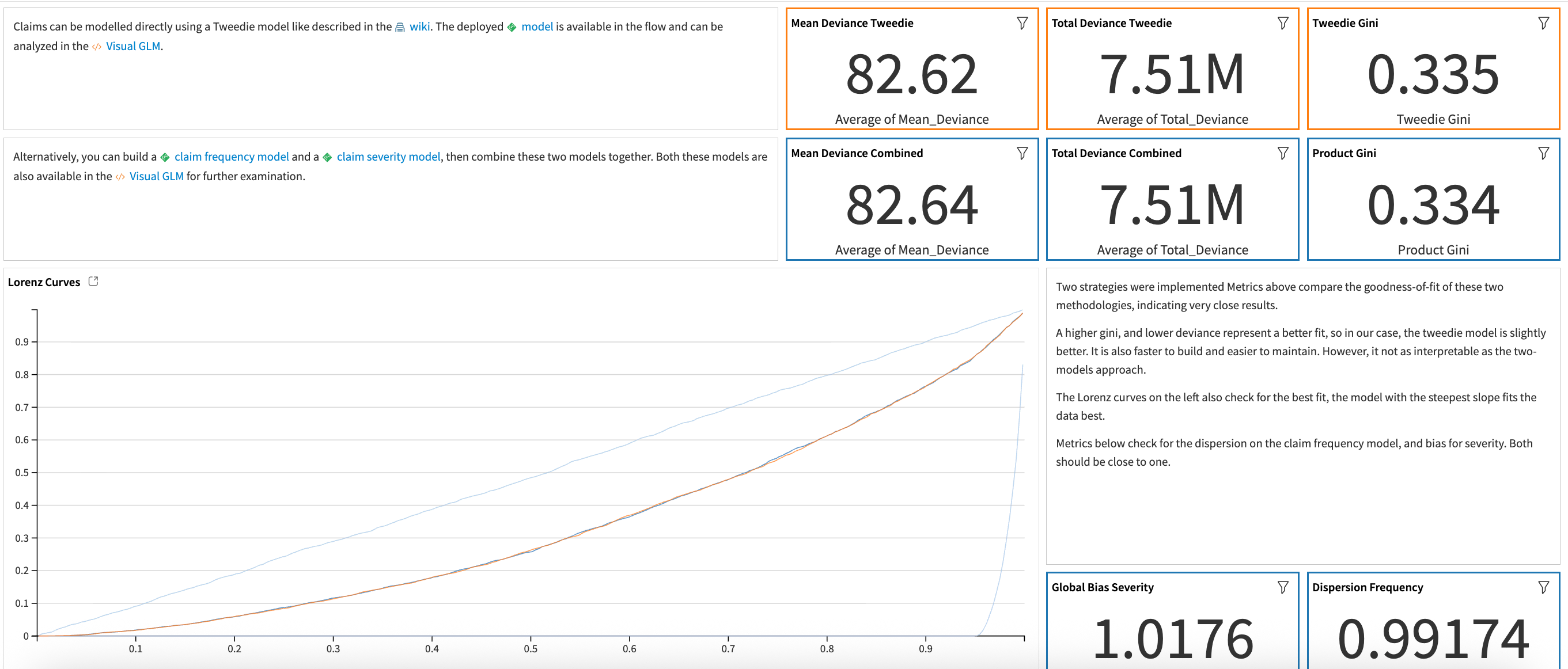
Two downstream Python recipes reproduce the diagnostic suite described in the wiki. The first calculates Tweedie deviance (variance power 1.5), Pearson Chi², dispersion, and global bias so actuaries can compare absolute fit. The second computes Lorenz curves for the compound, Tweedie, random, and oracle models, and derives the associated Gini coefficient using:

\[\text{Gini} = 1 - 2 \times \text{AUC}(\text{Lorenz})\]

The Model Comparison dashboard tab overlays these metrics so that teams can quickly see whether the interpretable compound approach or the faster Tweedie pipeline best meets their goals.

Deploy models to an API for real predictions

A deployed API service exposes all previously trained models. The API Flow zone regroups the three model endpoints (claim frequency, claim severity, and pure premium) along with the dataset that maps driver_age to spline basis functions, ensuring everything needed for scoring is versioned in one place. Because the feature engineering lives inside the Visual GLM scripts (or their feature-handling panels), no additional enrichment is required before building the service.

When configured on an API node, the claim_risk service accepts JSON payloads mirroring the claim_frequency dataset schema. Sample queries generated from that dataset help validate responses before promoting the service through the API Deployer. Once running, downstream systems can call any endpoint to obtain real-time predictions.

Enable claims teams with pre-built interactive dashboards

Note

For 11.4+ instances with UIF enabled, retraining of the model is necessary before starting the webapp for the first time to avoid a permission denied error.

In addition to the pre-defined model comparison analysis detailed above and visualized in the Model Comparison dashboard tab, this Solution comes with a pre-built webapp to allow for interactive model comparison. The interactive view available in the Interactive Model Comparison dashboard tab provides a view to explore model predictions, understand how each feature affects the models, and compare the model predictions.

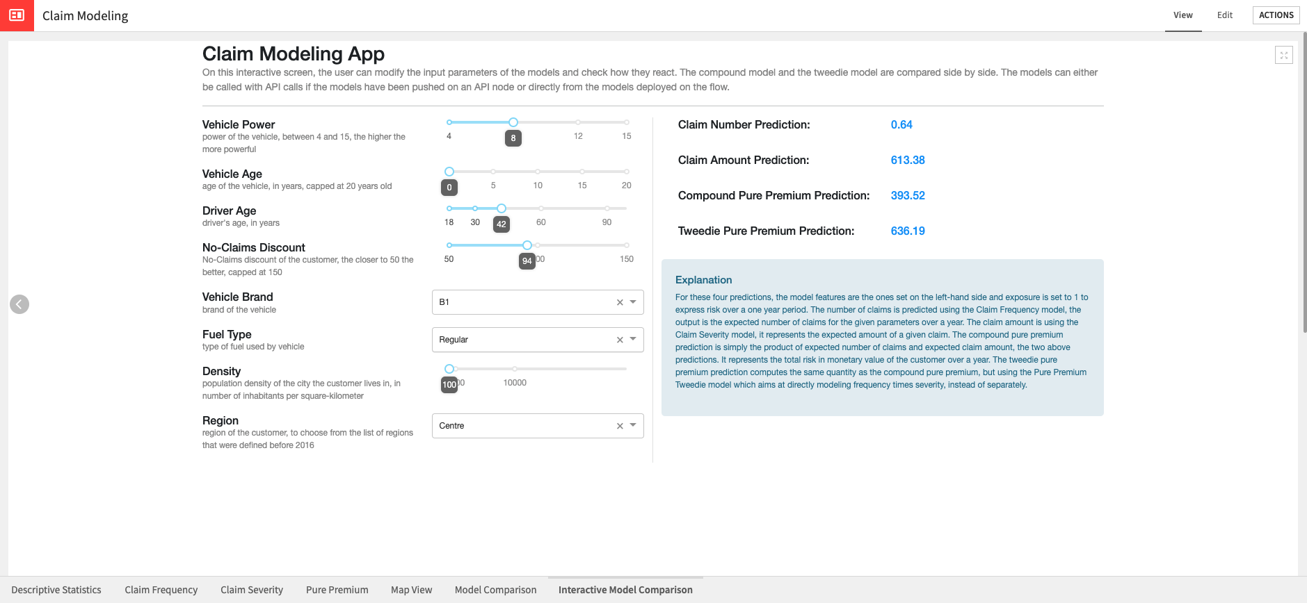
You can modify the impacting features using sliders or dropdown menus, triggering either an API call or direct scoring from the Flow (depending on configuration) to update four predictions: Claim Frequency, Claim Severity, Compound Pure Premium, and Tweedie Pure Premium. Exposure is fixed at 1 to express yearly risk, and ClaimNb is pinned to 1 when showing severity so the metric retains its standard definition. Area is intentionally hidden because EDA showed redundancy with density.

Two project variables control where the scoring happens:

• use_api - set to "True" to call the API service, or "False" to instantiate predictors locally from Flow models.

• api_node_url - points the webapp to the correct API node when use_api is true.

When local scoring is selected, a Python helper replicates the feature-processing logic once per interaction and then calls all three predictors so the dashboard stays responsive.

Reproducing these processes with minimal effort for your data

This project equips claims teams to create an insurance pricing model based on historical claim data using Dataiku and the GLM plugin. By creating a singular Solution that can benefit and influence the decisions of a variety of teams in a single organization, you can design smarter and more holistic strategies to leverage GLM pricing solutions, establish effective governance, and centralize pricing workflows without sacrificing agility.

This documentation has provided several suggestions on how to derive value from this Solution. Ultimately however, the “best” approach will depend on your specific needs and data. If you’re interested in adapting this project to the specific goals and needs of your organization, Dataiku offers roll-out and customization services on demand.