

Introduction#
Deep learning models are powerful tools for image classification, but they are difficult and expensive to create from scratch.
Dataiku provides several pre-trained deep learning models that you can use to classify images. You can also re-train a model to specialize it on a particular set of images.
In this tutorial, you will:
Classify images of healthy and diseased bean plant leaves using a pre-trained model.
Learn how to evaluate and fine-tune the model.
Use the model to classify new images.
Evaluate the model’s performance.
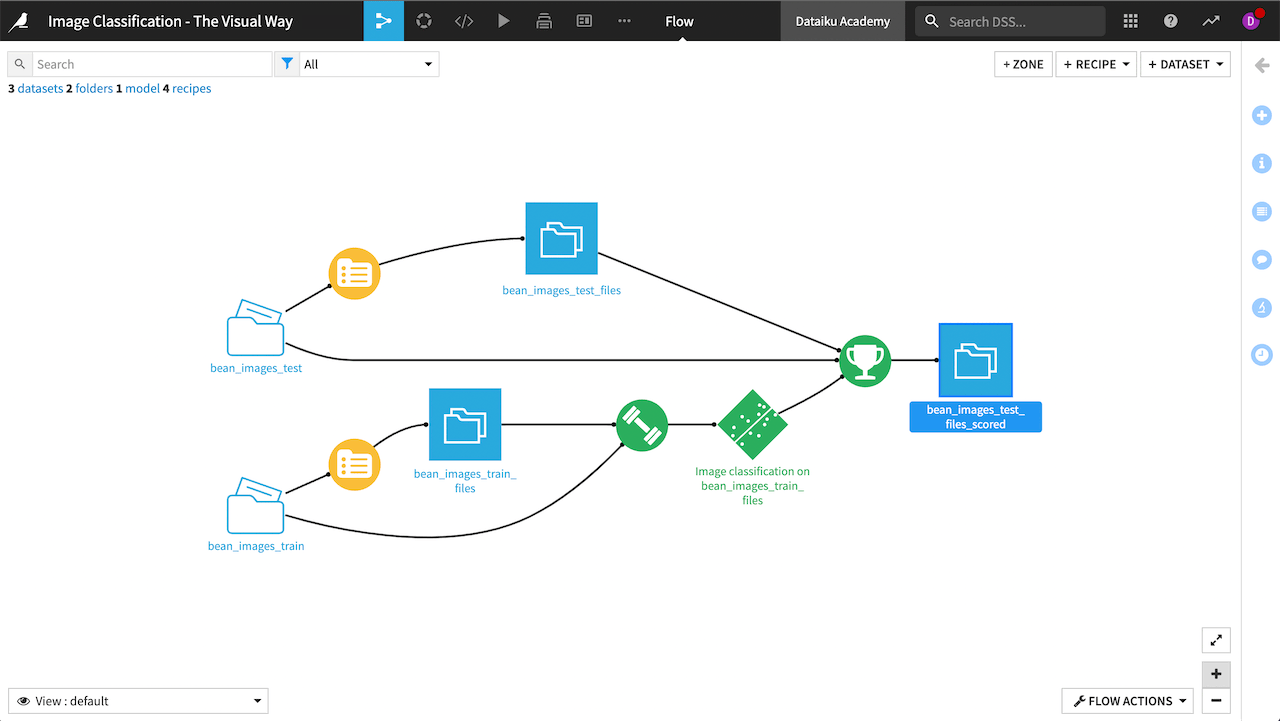
When finished, you’ll have built the Flow below.
Prerequisites#
A Dataiku instance (version 11.3 or above). Free edition is enough; Dataiku Cloud is not compatible.
A computer vision code environment, which you can set up in the Applications menu of Dataiku under Administration > Settings > Misc.
Create the project#
From the Dataiku homepage, select +New Project > DSS tutorials > ML Practitioner > Image Classification without Code.
Explore the data#
In the Flow, you’ll see two folders called bean_images_train and bean_images_test that contain the images for our classification model. The images are stored in managed folders, which is a requirement for running image classification models in Dataiku.

This dataset is from a project by the Artificial Intelligence Lab at Makerere University that uses image classification to help identify disease among bean crops in Uganda. The plants are classified as healthy or infected with bean rust or with angular leaf spot diseases.
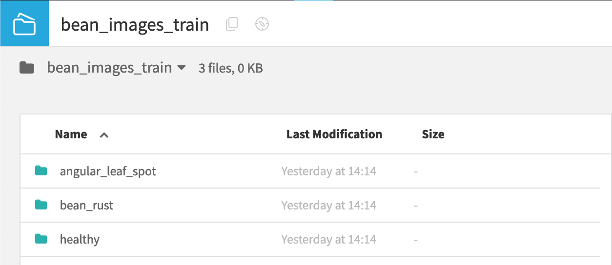
Take a moment to browse the files in the bean_images folder to get a sense of the images we’ll be classifying. The nearly 500 images are divided into three subfolders by class: healthy, bean_rust, and angular_leaf_spot.
The Flow also contains a folder called bean_images_test, with images we’ll use to test our model after training. That folder has a similar structure with three subfolders representing each image class.
Prepare the data for image classification#
Before we can create an image classifier, we need to build a tabular dataset that tells our model the file path where it can find each image. The dataset also will include the class for each image, which will be the target for our model to predict. We’ll do this using the List Contents recipe, which lists all files in a folder, their file paths, and other information.
With the bean_images_train folder highlighted, go to the Actions menu on the right panel and select the List Contents recipe from Visual recipes.
In the New List Folder Contents recipe dialog, create the recipe with the default settings and name bean_images_train_files.
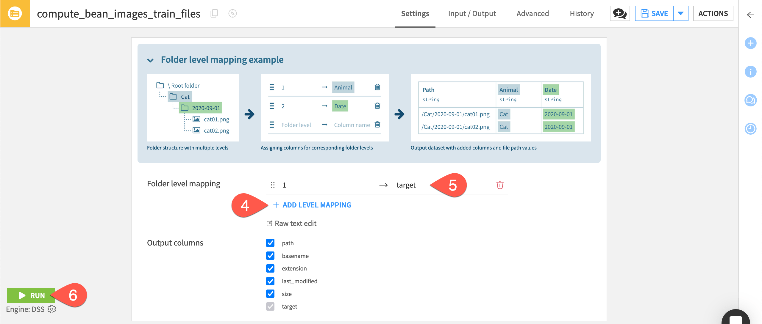
In the recipe Settings tab, select +Add Level Mapping and set the Folder level to
1, and the Column name totarget.This creates a column called target that contains the name of the folder where each image is located, which is the image’s category, or class.
Run the recipe.
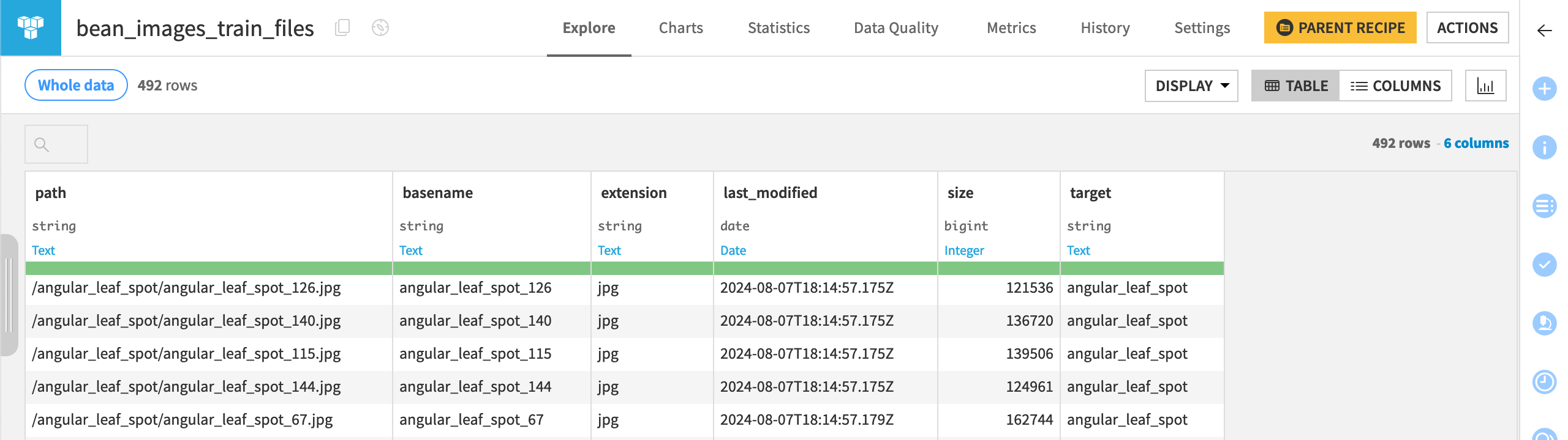
The resulting table bean_images_train_files contains 492 rows with the name and file path of each image, along with a column called target where each image is labeled as healthy, bean_rust, or angular_leaf_spot.
Fine-tune a pre-trained model#
After preparing the data, we are ready to use one of the pre-trained image classification models in Dataiku.
Note
Before building an image classification model, you must set up a specific code environment. Go to Administration > Settings > Misc. In the section DSS internal code environment, create an Image classification code environment by selecting your Python interpreter and clicking on Create the environment. Dataiku will install all the required packages for image classification and add the new code environment to the Code Envs tab.
Create the model#
In this section, we’ll create a model in the Lab, and later we’ll deploy it in the Flow.
In the Flow, highlight the bean_images_train_files dataset and go to the Lab, then choose Image Classification.
The next window asks you to define the model’s target, or what categories it will predict. Choose the target column.
Select the bean_images_train folder in the Image folder dropdown to tell the model where to find the images for training.
Name your model or leave the default name and select Create.
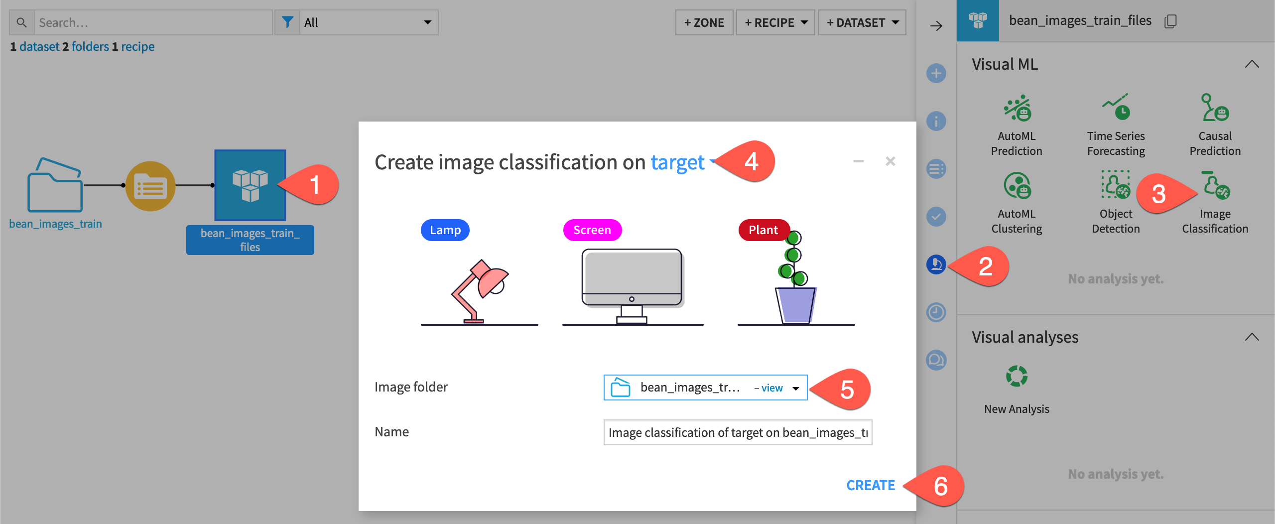
Dataiku creates the image classification model and adds it to the Lab, then navigates to the model Design tab where you can preview images and settings. Before training the model, let’s review the input and settings.
Check the model settings#
The Basic > Target panel shows the Target column and Image location we input when creating the model. It also recognizes the Path column so the model can find each image. Double-check that these settings are correct.
Under Target classes, the model automatically recognizes that we have created a classification task with three classes of healthy or diseased bean plants. You can preview the images and filter them by selecting each class in the bar chart.
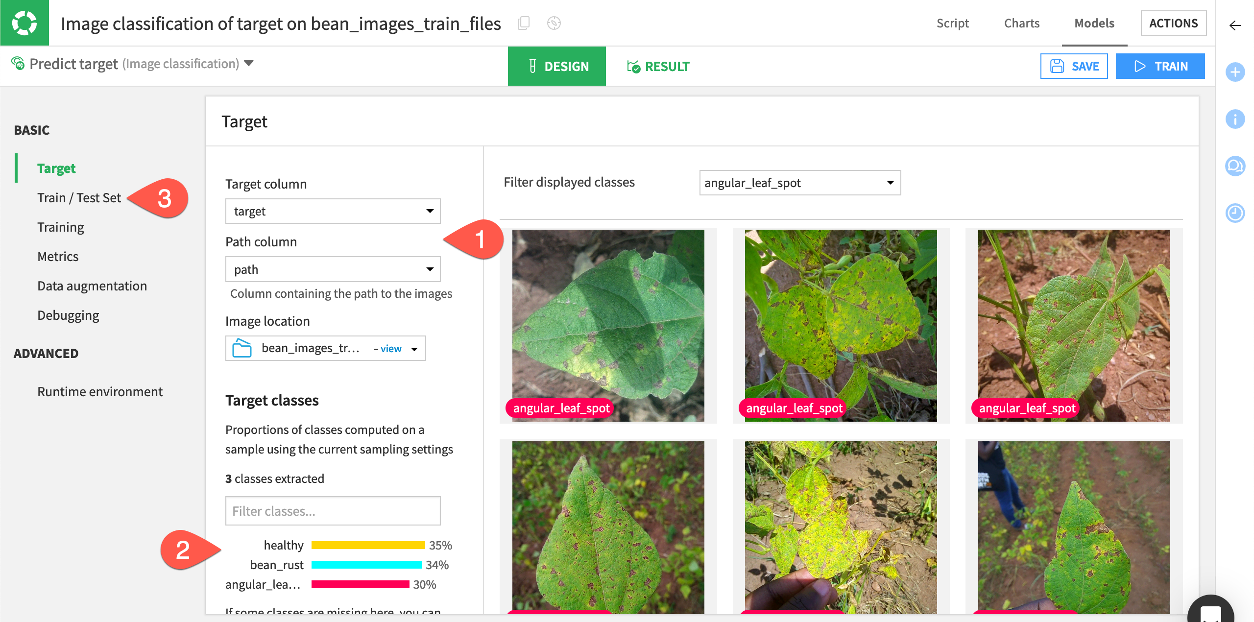
Dataiku will also automatically split the images into training and validation sets so the model can continually test its performance during the training phase. You can see these settings under Basic > Train/Test Set. This panel also contains sampling settings, which you might want to change when using larger datasets.
Choose a pre-trained model#
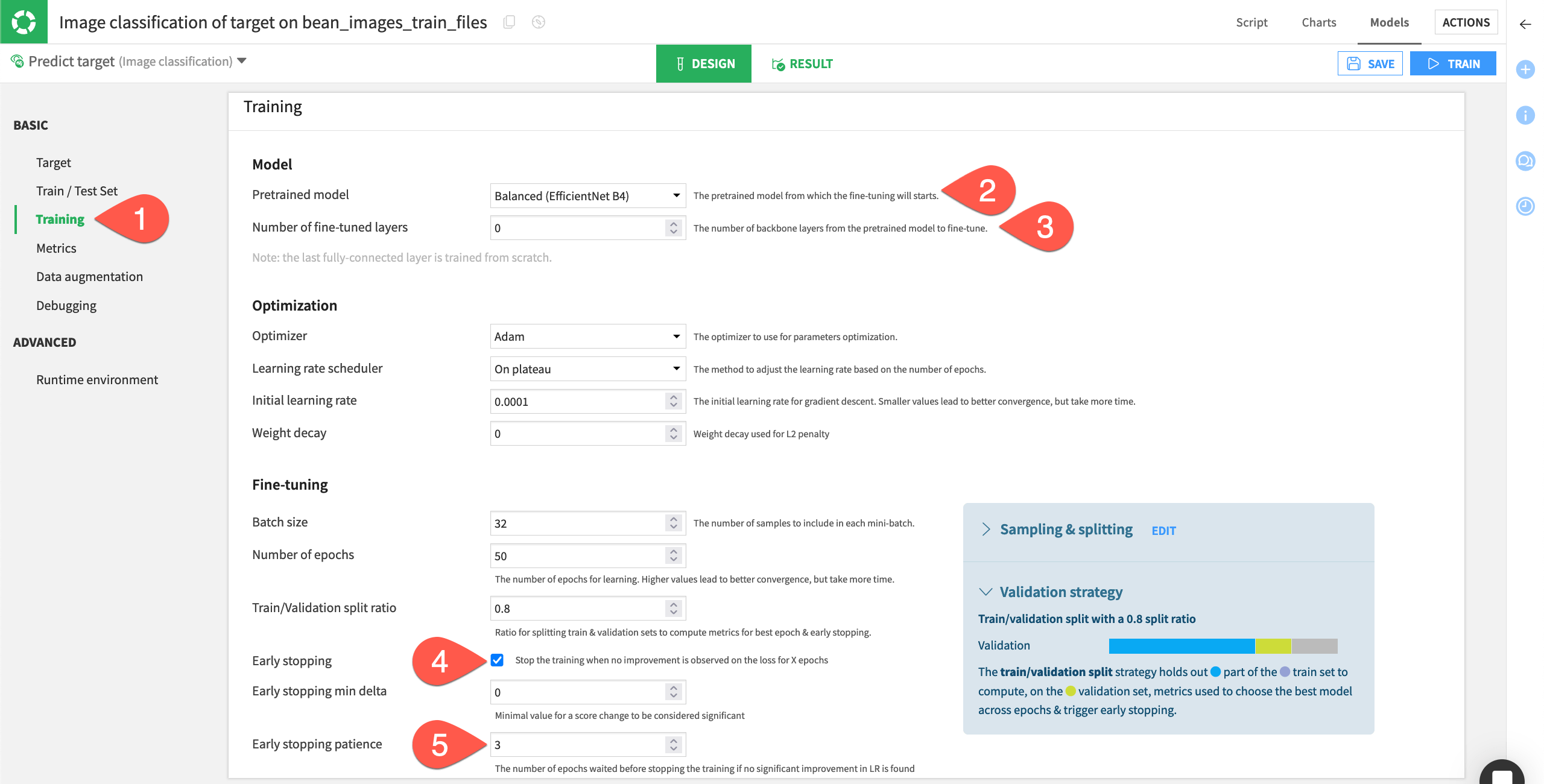
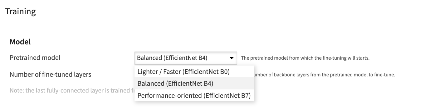
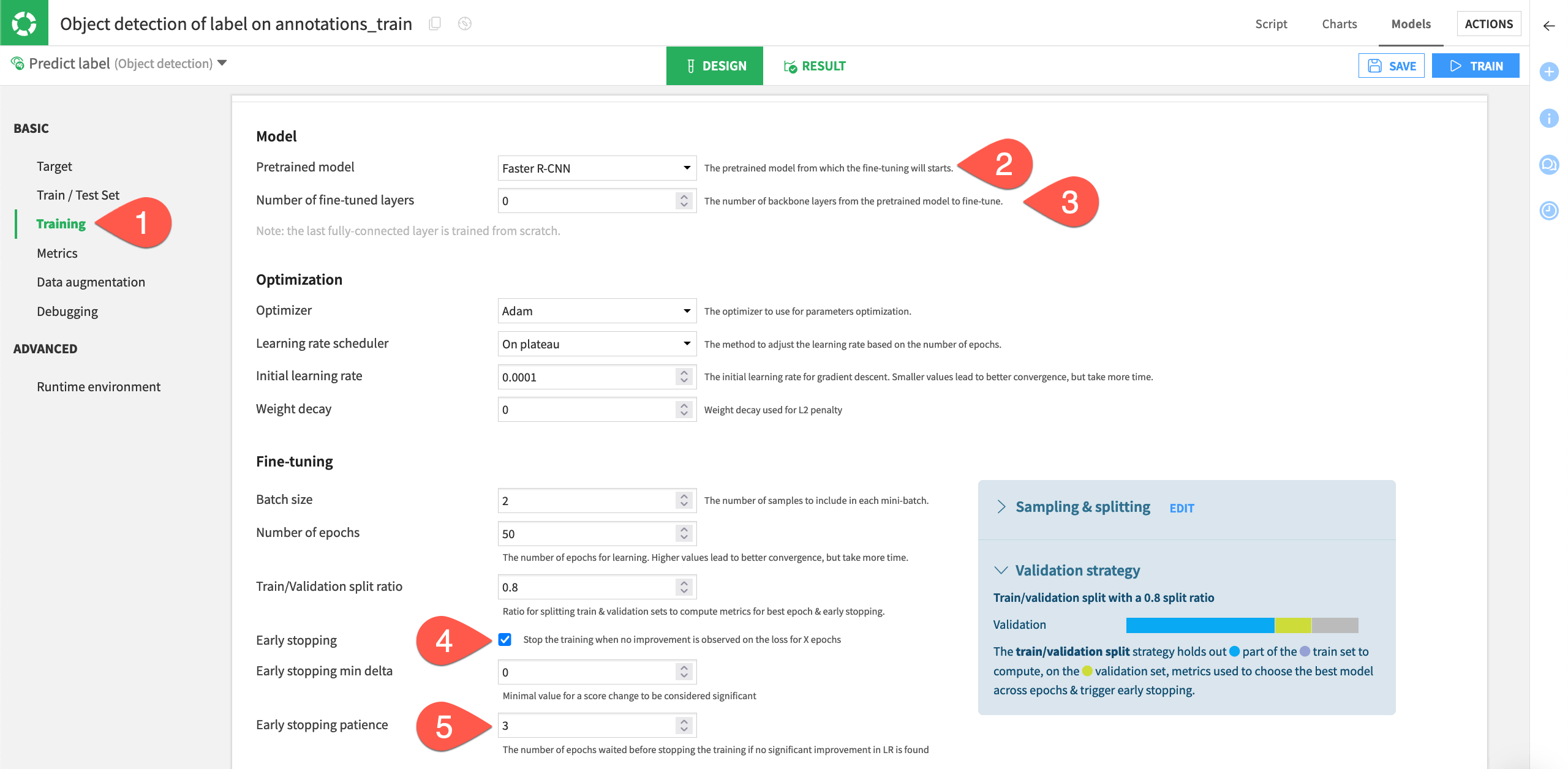
Dataiku provides three pre-trained neural networks that are widely used and considered industry standards. You can see all the models and choose one to use in the Design tab under Basic > Training > Model.
EfficientNet B0: Efficiency-oriented
EfficientNet B4: Balanced between efficiency and performance
EfficientNet B7: Performance-oriented
Balanced (EfficientNet B4) is the default model, and we will use it in this tutorial.
Also in the Model section, you can specify how many layers of the model to retrain on your images. Convolutional neural networks (CNN) have many different layers that are pre-trained on millions of images. Retraining the final layer or final few layers helps the model learn on your specific images.
Dataiku’s models always retrain the final layer, also called classifier layer, to adapt it to the use case at hand. The default setting of 0 under Number of fine-tuned layers means one layer will be fine-tuned. Inputting 1 here means that two layers will be finetuned, and so on. Adding fine-tuned layers can increase performance but also increases processing time. We will use the default of 0.
In the Optimization and Fine-tuning sections, values are set to industry standards, and in most cases you will not change these.
For purposes of this tutorial, if you want the model to finish training more quickly, make sure Early stopping is selected and change the Early stopping patience to 3.
This means the model will stop cycling through images if it does not detect any performance improvement after three cycles, or epochs. We’ll discuss epochs and early stopping patience further in the Concept | Optimization of image classification models lesson.
Train the model#
When you are finished viewing the settings, select Save.
Click Train at the top right to begin training the model.
In the window, give your model a name or use the default and select Train.
Note
If your Dataiku instance is running on a server with a GPU, you can activate the GPU for training so the model can process much more quickly. Otherwise, the model will run on CPU and the training will take longer.
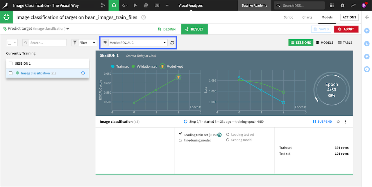
Model training can take time depending on your computer’s memory capacity. During training, you can view the chart in the Result tab to track the performance of your model at the end of each epoch. The default metric to evaluate and maximize the model’s performance is ROC AUC, or area under the curve, but other metrics such as Precision or Accuracy are available in the Metric dropdown above the chart.
Tip
You can review the concepts behind ROC AUC and other various metrics in Concept | Model evaluation.
After training completes, you can assess the performance of your model before deploying it to the Flow.