Tutorial | Window recipe

The Window recipe utilizes advanced grouping to apply aggregate calculations to each row in your dataset. Let’s practice using different windows to show how they affect these calculations.

Get started

Objectives

In this tutorial, you will:

• Learn how to configure different windows in the recipe.

• Find cumulative sums for each row.

• Calculate windows based on a range of rows.

• Calculate windows based on a range of values.

Prerequisites

To complete this tutorial, you’ll need the following:

• Dataiku 12.0 or later.

Create the project

Dataiku 13.3+Dataiku Pre-13.3

1. From the Dataiku Design homepage, click + New Project.

2. Select Learning projects.

3. Search for and select Window Recipe.

4. Click Install.

5. From the project homepage, click Go to Flow (or g + f).

Note

You can also download the starter project from this website and import it as a zip file.

You’ll next want to build the Flow.

1. Click Flow Actions at the bottom right of the Flow.

2. Click Build all.

3. Keep the default settings and click Build.

Use case summary

Let’s say we’re a financial company that uses some credit card data to detect fraudulent transactions.

The project comes with three datasets, described in the table below.

Dataset	Description
tx	Each row is a unique credit card transaction with information such as the card that was used and the merchant where the transaction was made. It also indicates whether the transaction has either been: Authorized (a score of 1 in the authorized_flag column) Flagged for potential fraud (a score of 0)
merchants	Each row is a unique merchant with information such as the merchant’s location and category.
cards	Each row is a unique credit card ID with information such as the card’s activation month or the cardholder’s FICO score (a common measure of creditworthiness in the US).

Create the Window recipe

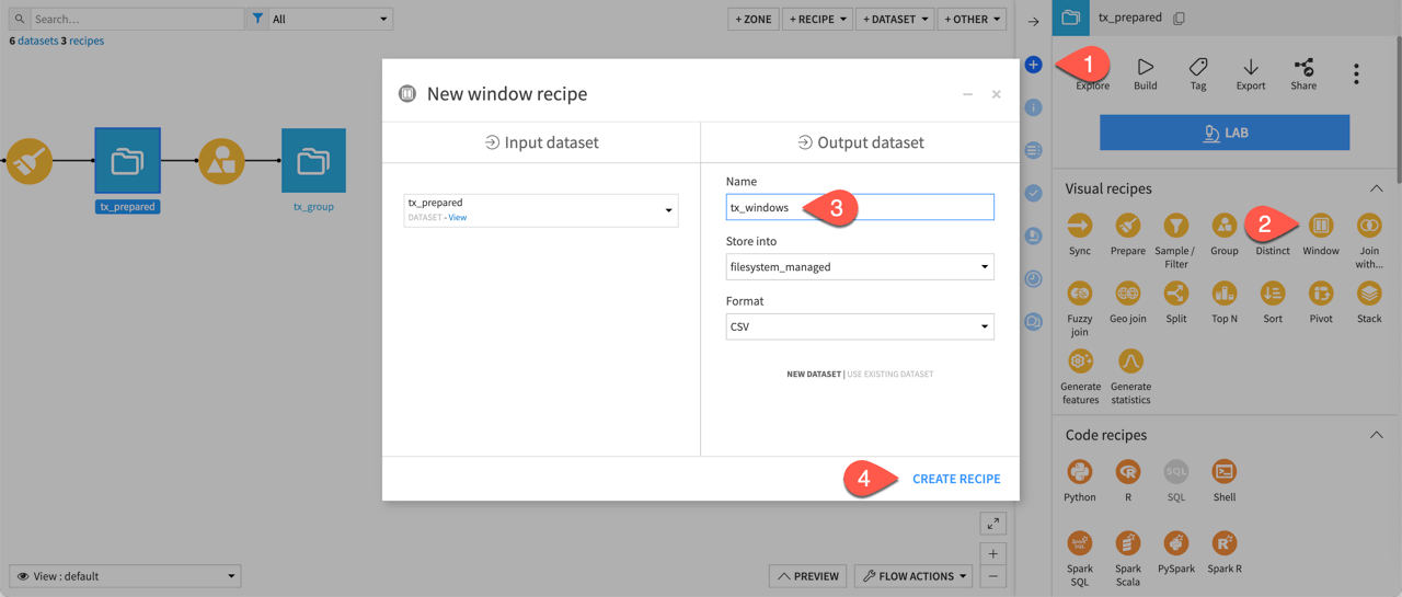
We’ll create a Window recipe from the tx_prepared dataset.

1. From the Flow, select the tx_prepared dataset and click the Actions icon (+) from the right panel to open the Actions tab.

2. Under the Visual Recipes section, click on Window.

   The New window recipe window opens.

3. Change the output name to tx_windows.

4. Click Create Recipe.

Use an undefined window frame

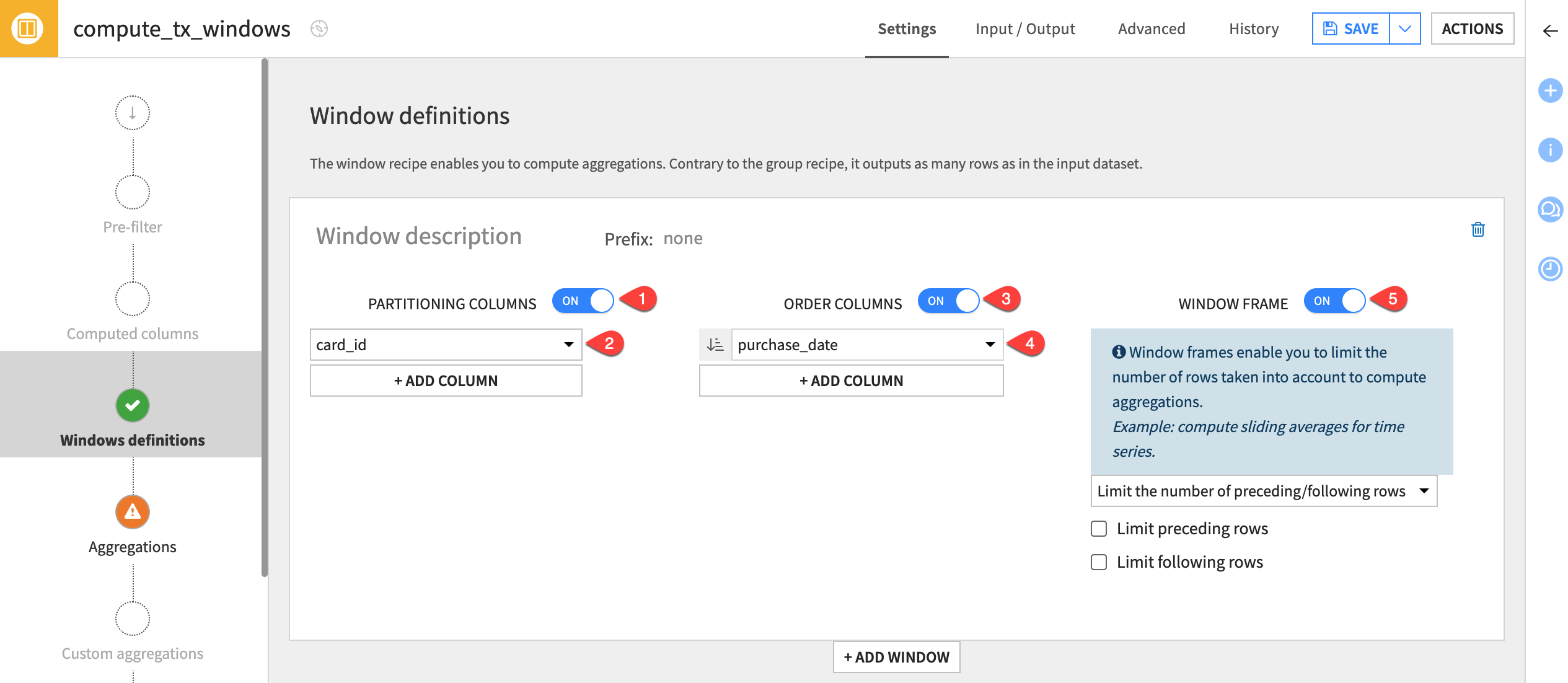
Let’s practice first by using an undefined window — that is, one without bounds. In this case, we’ll compute the sum of card purchases by card_id, ordered by purchase_date.

1. In the Window definitions step, toggle on Partitioning Columns.

2. Choose card_id from the dropdown menu.

3. Toggle on Order Columns.

4. Choose purchase_date from the dropdown menu.

5. Toggle on Window Frame, but make no further adjustments.

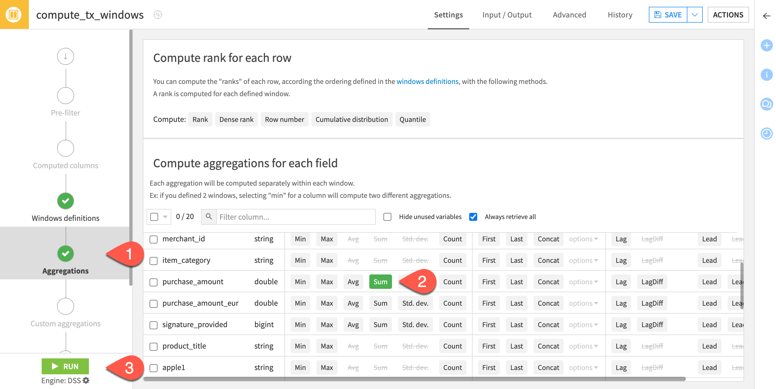
Next, we’ll choose the correct aggregations for our window.

1. Navigate to the Aggregations step.

2. Enable Sum on the purchase_amount column.

3. Run the recipe.

Interpret the output

Now we will interpret the recipe output. For clarity, we’ll also filter the results for a specific card_id since that is the partitioning column.

1. Open the output tx_windows dataset. You’ll see a new column purchase_amount_sum in the dataset.

2. For further simplicity, near the top right, click Display > Select displayed columns.

3. Keep only the following five columns: id, purchase_date, card_id, purchase_amount, and purchase_amount_sum.

4. Click the column dropdown header of card_id.

5. Click Filter.

6. Select a frequent card_id value, such as C_ID_003e56029c.

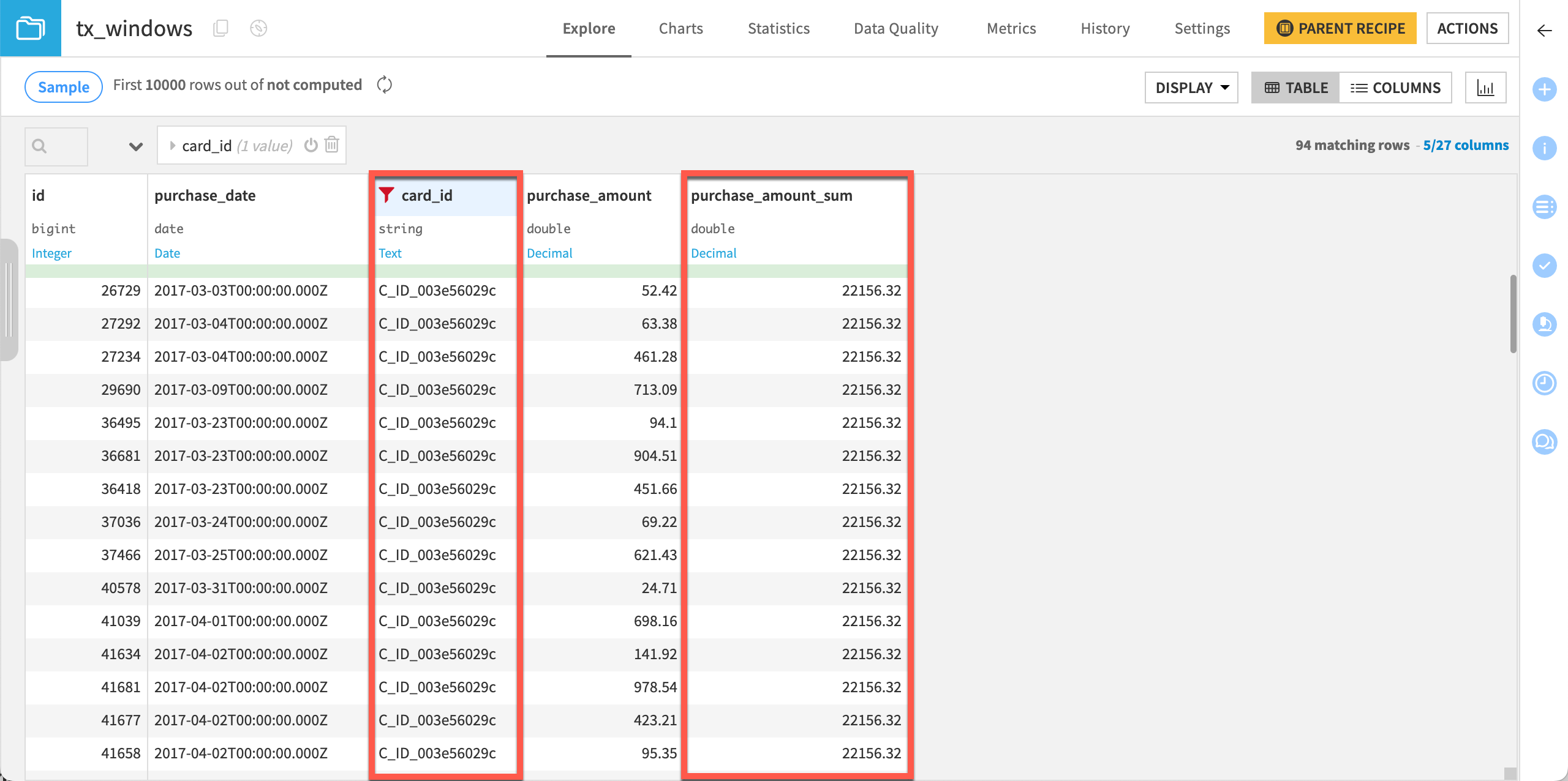
You should see that the purchase_amount_sum is the same for each row! This is because the window frame included all purchase amounts for that credit card in the aggregation.

Find the cumulative sum

This next exercise involves finding the cumulative sum of purchase amounts for each row. In this case, we want to find the sum of all purchase amounts of a credit card before and including each purchase date.

1. Click Parent Recipe to reopen the Window recipe.

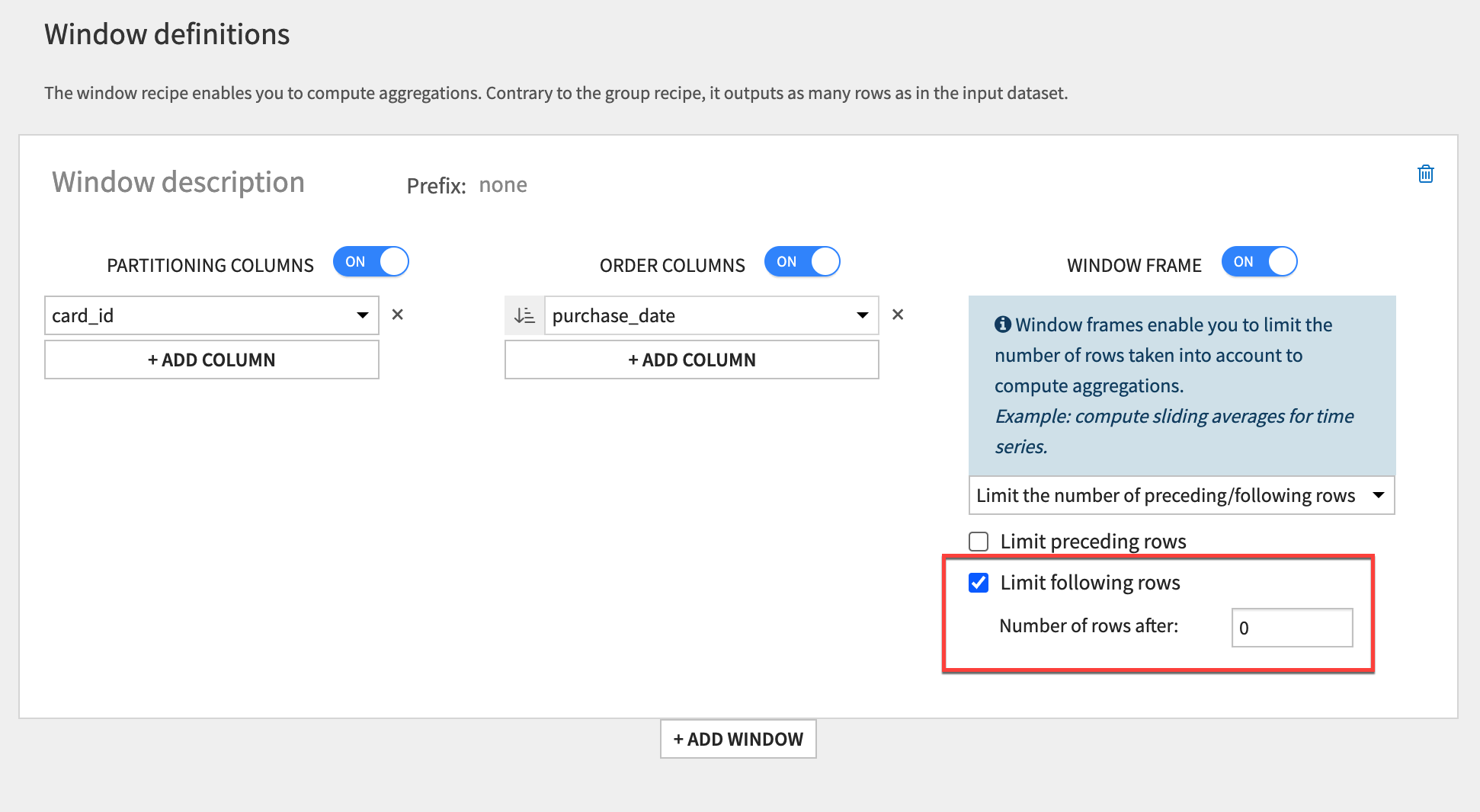
2. Under the Window Frame settings, select the Limit following rows checkbox and leave the number of rows as 0. This will set the window to be all rows before and including the current row.

3. Run the recipe and open the output dataset.

Now, the purchase_amount_sum varies for each row. Notice that as the purchase dates increase, the sum also increases. This will be the case if there are no negative purchase amount values, such as for a refund given.

Use a range of rows

Now we will set the window to limit the previous rows in addition to the following rows.

1. In the top left corner, click Parent Recipe to reopen the Window recipe.

2. Select the Limit preceding rows checkbox.

3. Set the number of rows before to 5 and the number of rows after to -1. This will make the window include five rows before the current row, excluding the current row.

4. Run the recipe and open the output.

In this dataset, the purchase_amount_sum doesn’t necessarily increase with time. This is because the window is not always increasing — after the first five rows in the dataset, it is always five rows in size, leaving out earlier rows from the window frame.

Use a value range

So far, we’ve been defining our window relative to the rows in the dataset. However, we can also define the window frame relative to the values in a column. In this case, we’ll be limiting our window frame by a range of days from the purchase_date ordering column.

1. Click Parent Recipe to reopen the Window recipe.

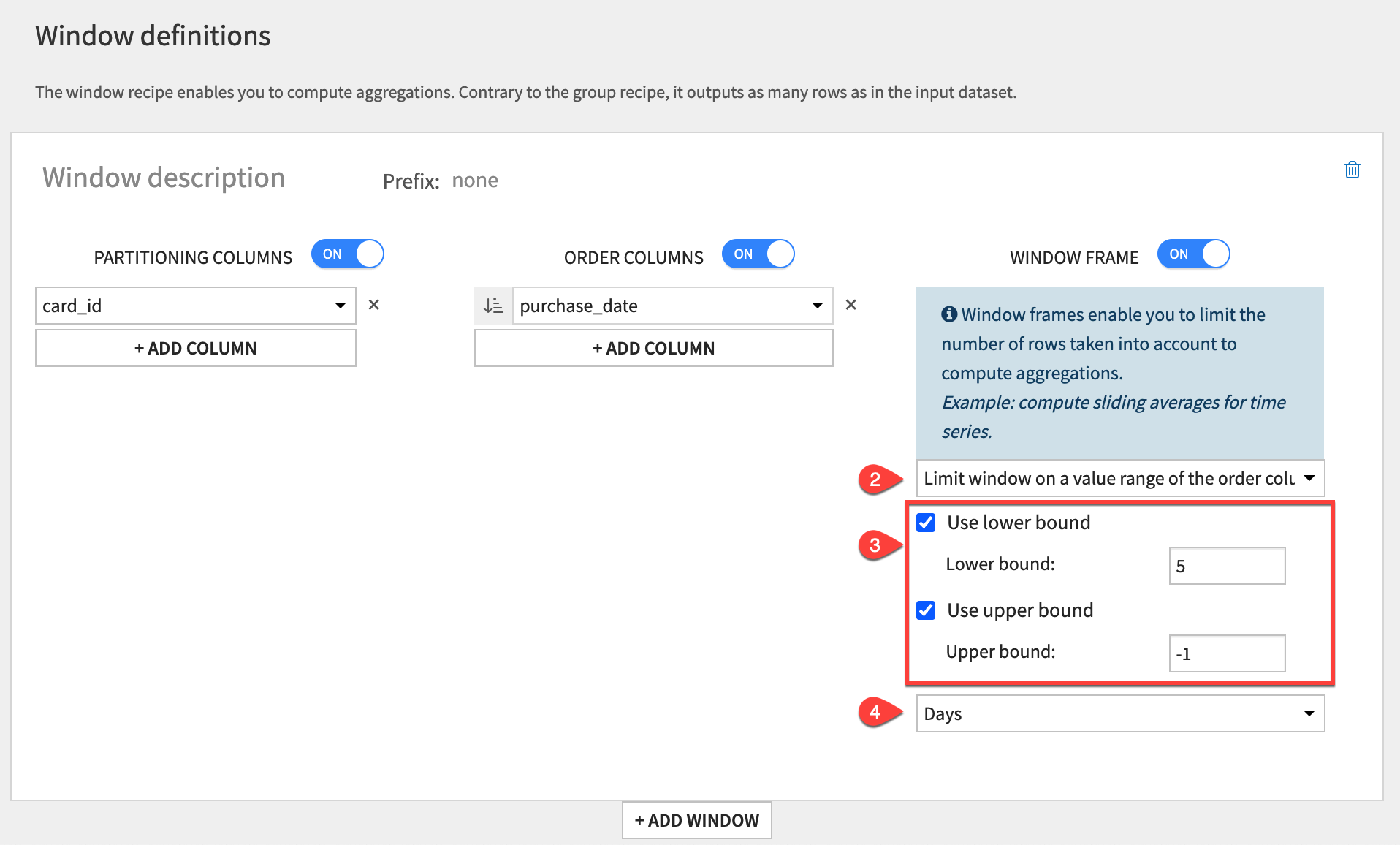
2. Under Window Frame, select Limit window on a value range of the order column.

3. Make the lower bound 5 and the upper bound -1.

4. Change the window unit to Days. This will make the window include records that are 5 days before the target row’s date, excluding the target row.

5. Run the recipe and open the output.

This is the first output we’ve seen with empty values after the first row in the purchase_amount_sum column. Why did this happen?

Since we did not use a range of rows for our window, there was no guarantee that there would be any records for the time period before the current record. For example, in the row where the ID equals 36418, the purchase_amount_sum value is empty because there were no purchases from that card for the five days before 2017-03-23.

Compute lag

So far, we haven’t changed much in the Aggregations step of the recipe. Let’s try out some different options here.

1. Click on Parent Recipe to return to the Window recipe.

2. Navigate to the Aggregations step.

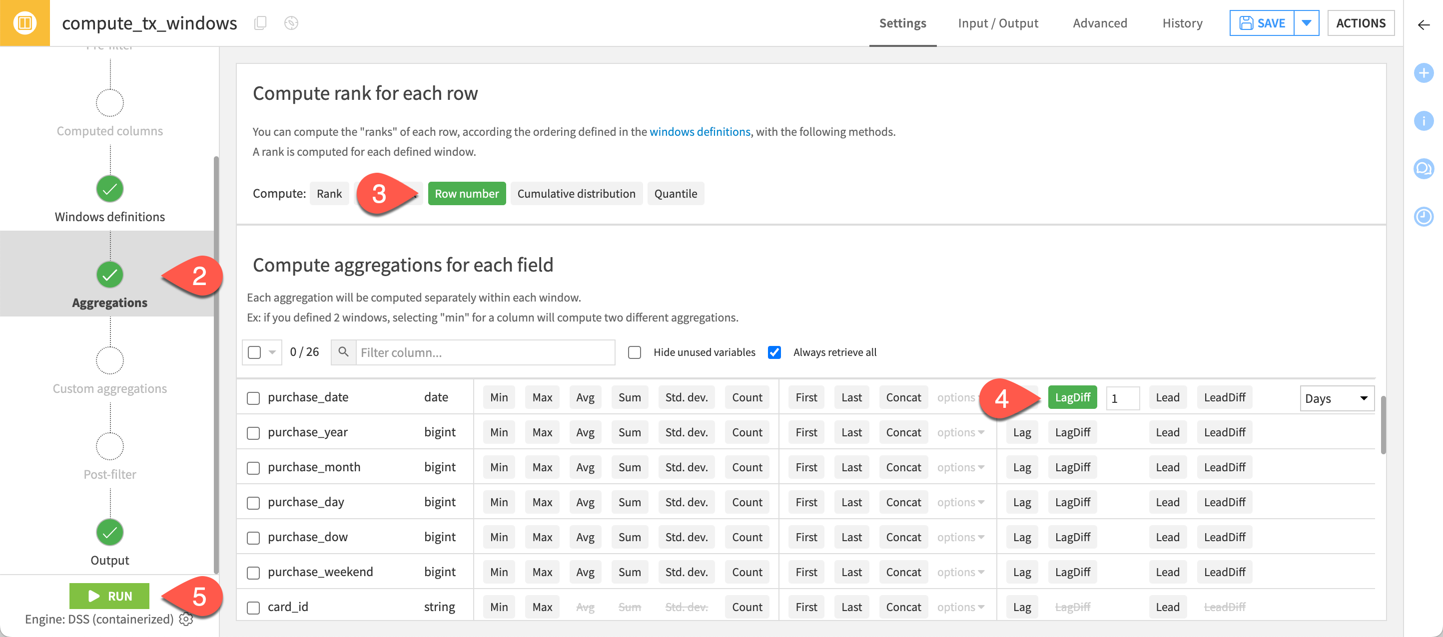
3. Under Compute rank for each row, turn on Row number.

4. Under Compute aggregations for each field, enable LagDiff on purchase_date with a value of 1 with the unit Days.

5. Run the recipe and open the output.

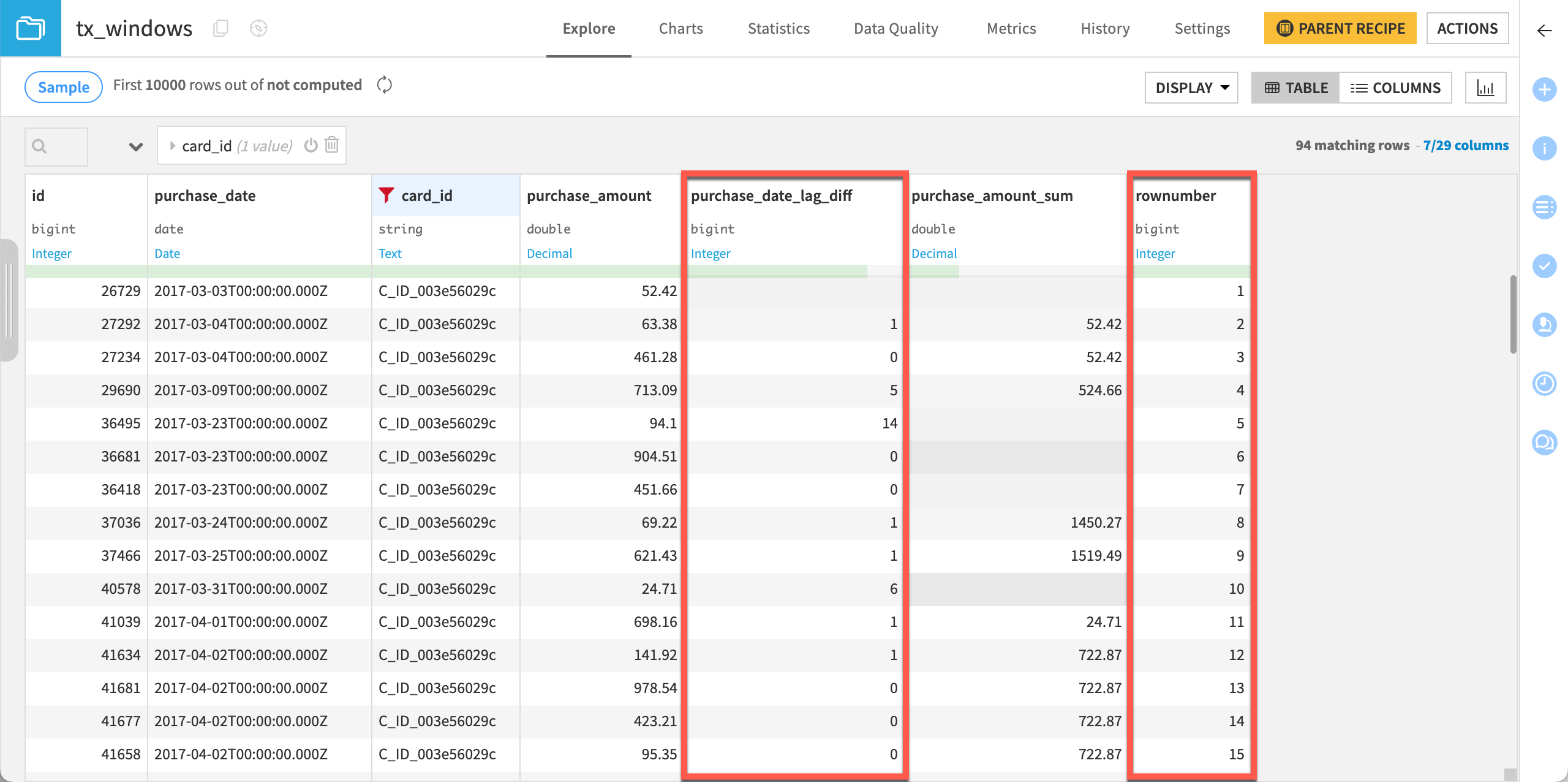
First, look at the rownumber column. In this case, we can interpret these values as the count of purchases on this card to date.

Next, look at the purchase_date_lag_diff column. These values show the difference in days between consecutive card purchases. As you can see, even though our window frame is defined by column values, the LagDiff is computed using the previous row (not previous day).

Tip

If we had wanted to rename the columns to better match their meanings, we could have done so in the Output step of the recipe.

What’s next?

You just used the Window recipe to enrich your dataset with new insights, while keeping the structure of the dataset intact.

See also

For more information on this recipe, see also the Window: analytics functions article in the reference documentation.

Another useful data transformation to test out can be explored in Tutorial | Top N recipe!