Tutorial | File-based partitioning

About partition redispatch

Partitioning refers to the splitting of a dataset along meaningful dimensions. Each partition contains a subset of the dataset. With partitioning, you can process different portions of a dataset independently.

There are two types of partitioning in Dataiku:

• File-based partitioning

• Column-based partitioning

If you are using a file system connection and your files do not map directly to partitions, you can still partition your dataset using Partition Redispatch. For example, you might have a collection of files containing unordered timestamped data where you want to partition on the date.

You can go from having a non-partitioned dataset to a partitioned dataset, using the Partition Redispatch feature. With Partition Redispatch, Dataiku reads the whole dataset once, sending each row to exactly one partition, depending on the values of its columns.

For example, if you decide to partition by purchase date and several rows of your dataset have a value of “2017-12-20” for the purchase date, those rows are assigned to the “2017-12-20” partition.

All datasets based on files can be partitioned. You can partition a file-based dataset by defining a pattern that maps each file to a single partition.

Let’s use the Partition Redispatch feature to partition a non-partitioned dataset.

Get started

In this tutorial, we will modify a completed Flow dedicated to the detection of credit card fraud. Our goal is to be able to predict whether or not a transaction is fraudulent based on the transaction subsector (e.g., insurance, travel, and gas) and the purchase date.

Objectives

Our Flow should meet the following business objectives:

• Be able to create time-based computations.

• Train a partitioned model to test the assumption that fraudulent behavior is related to merchant subsector, which is discrete information.

To meet these objectives, we will work with both discrete and time-based partitioning. Specifically, by the end of the lesson, we will accomplish the following tasks:

• Partition a dataset for the purpose of optimizing a flow and creating targeted features.

• Apply the Partition Redispatch feature to a non-partitioned dataset creating both time-based and discrete-based dimensions.

• Propagate partitioning in a Flow.

• Stop partitioning in a Flow.

Create the project

Dataiku 13.3+Dataiku Pre-13.3

1. From the Dataiku Design homepage, click + New Project.

2. Select Learning projects.

3. Search for and select Partitioning: File-Based.

4. Click Install.

5. From the project homepage, click Go to Flow (or g + f).

Note

You can also download the starter project from this website and import it as a zip file.

Use case summary

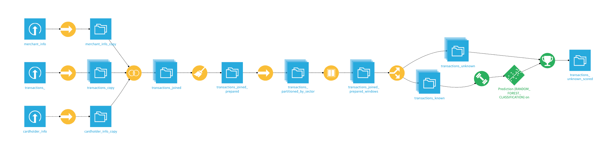
The Flow contains the following datasets:

• cardholder_info contains information about the owner of the card used in the transaction process.

• merchant_info contains information about the merchant receiving the transaction amount, including the merchant subsector (subsector_description).

• transactions_ contains historical information about each transaction including the purchase_date.

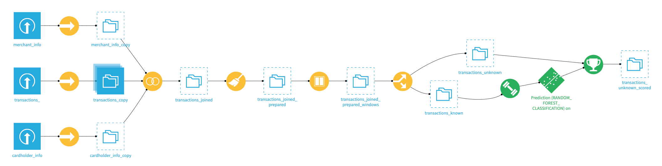
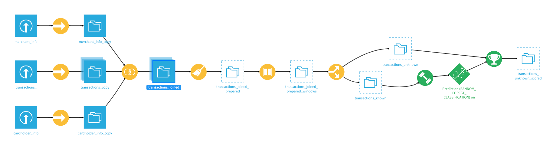
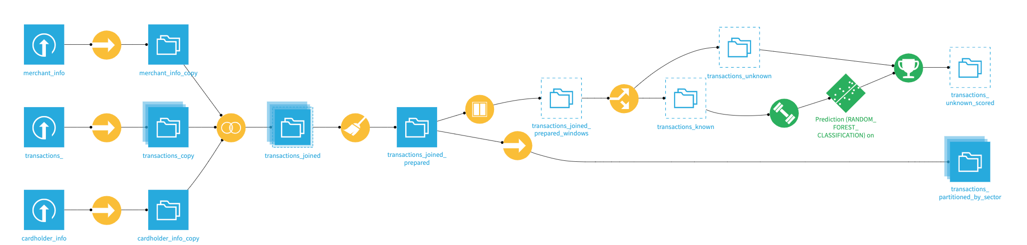
The final pipeline in Dataiku is shown below.

Build a time-based partitioned dataset

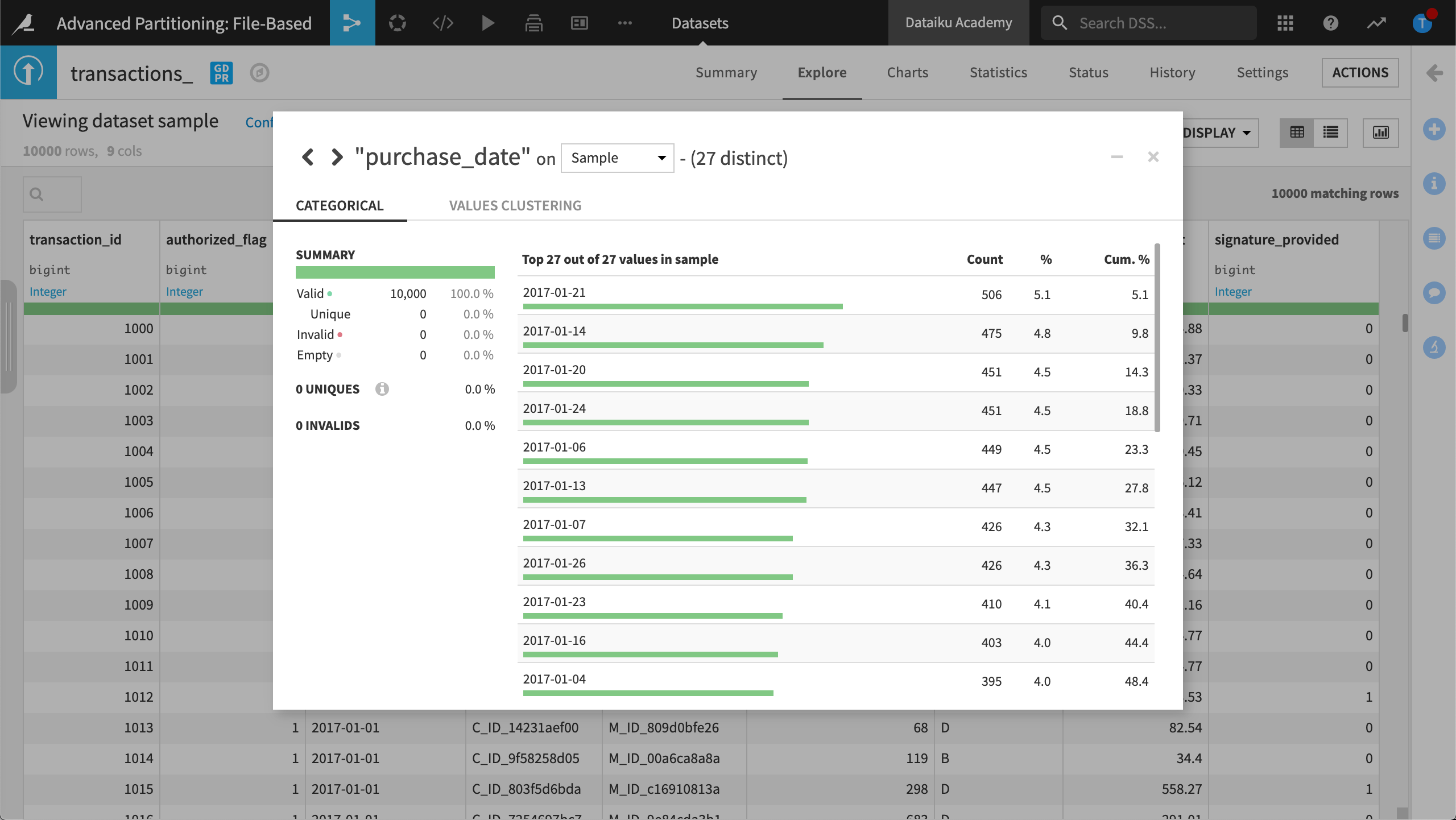
In this section, we will partition the dataset, transactions_copy, using the purchase_date dimension. The column, purchase_date, contains values representing the date of the credit card transaction.

Create a partitioned output

We want to partition the transactions_copy dataset by “day” using information in the purchase_date column.

We’ll use the Partition Redispatch feature of the Sync recipe. To make use of the Partition Redispatch feature, we must first create a partitioned output:

1. Open the Sync recipe that was used to create transactions_copy.

2. Run the recipe so that the dataset is built.

3. Open transactions_copy.

4. View the Settings page and click the Partitioning tab.

5. Click Activate Partitioning then Add Time Dimension.

6. Name the Dimension purchase_date, and set the Period to Day.

7. In Pattern, type %Y-%M-%D/.*.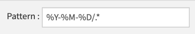

   

   When our dataset is stored on the filesystem, Dataiku uses this pattern to write the data on the filesystem connection. To find out more, see Concept | Partitioning by pattern.

8. Click SAVE.

   Dataiku informs you that it needs to fix the dependencies where this dataset is used as the input to a recipe.

   

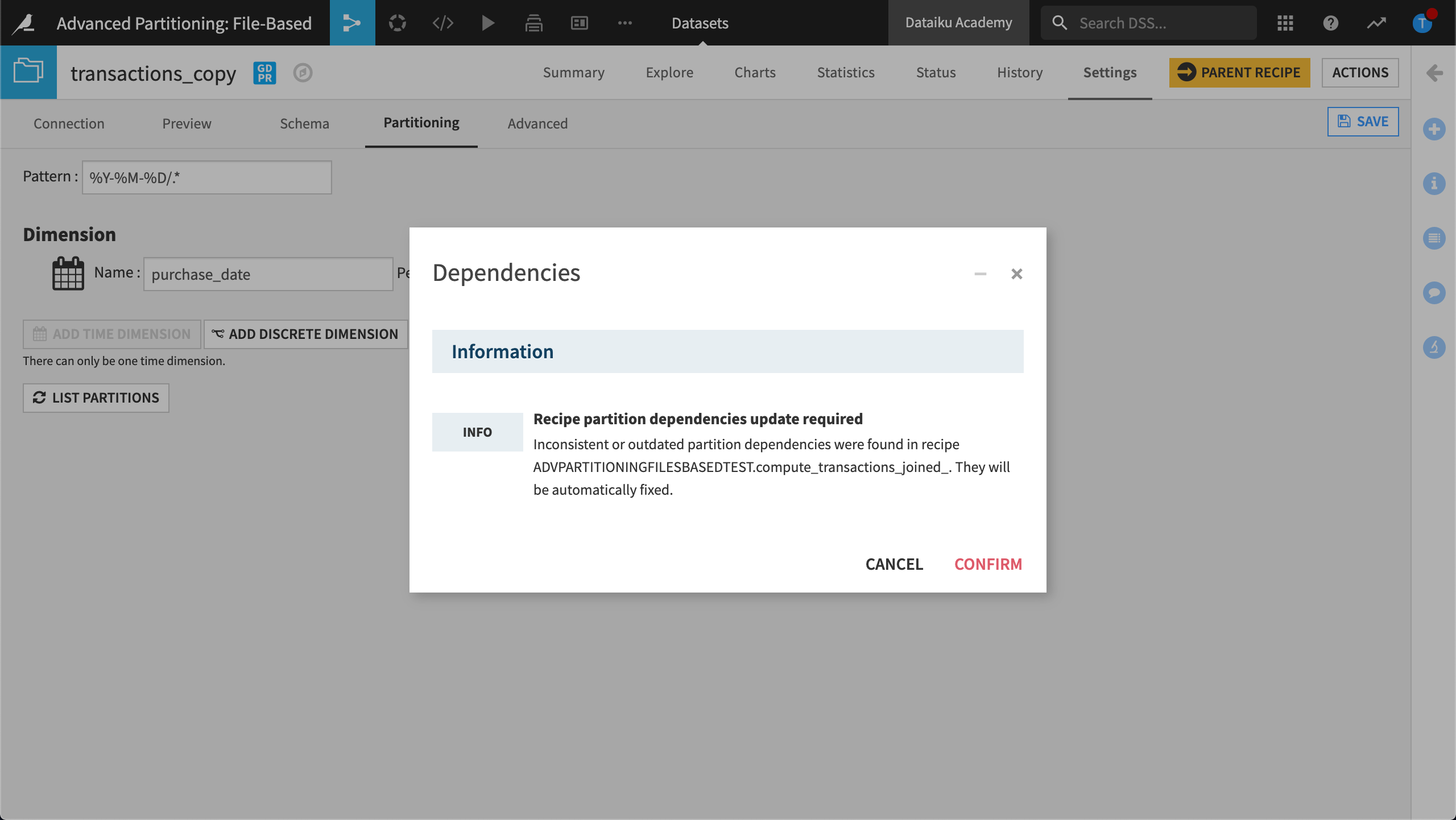
9. Click Confirm and return to the Flow.

The transactions_copy dataset now has a layered icon indicating it is partitioned.

Configure the Sync recipe

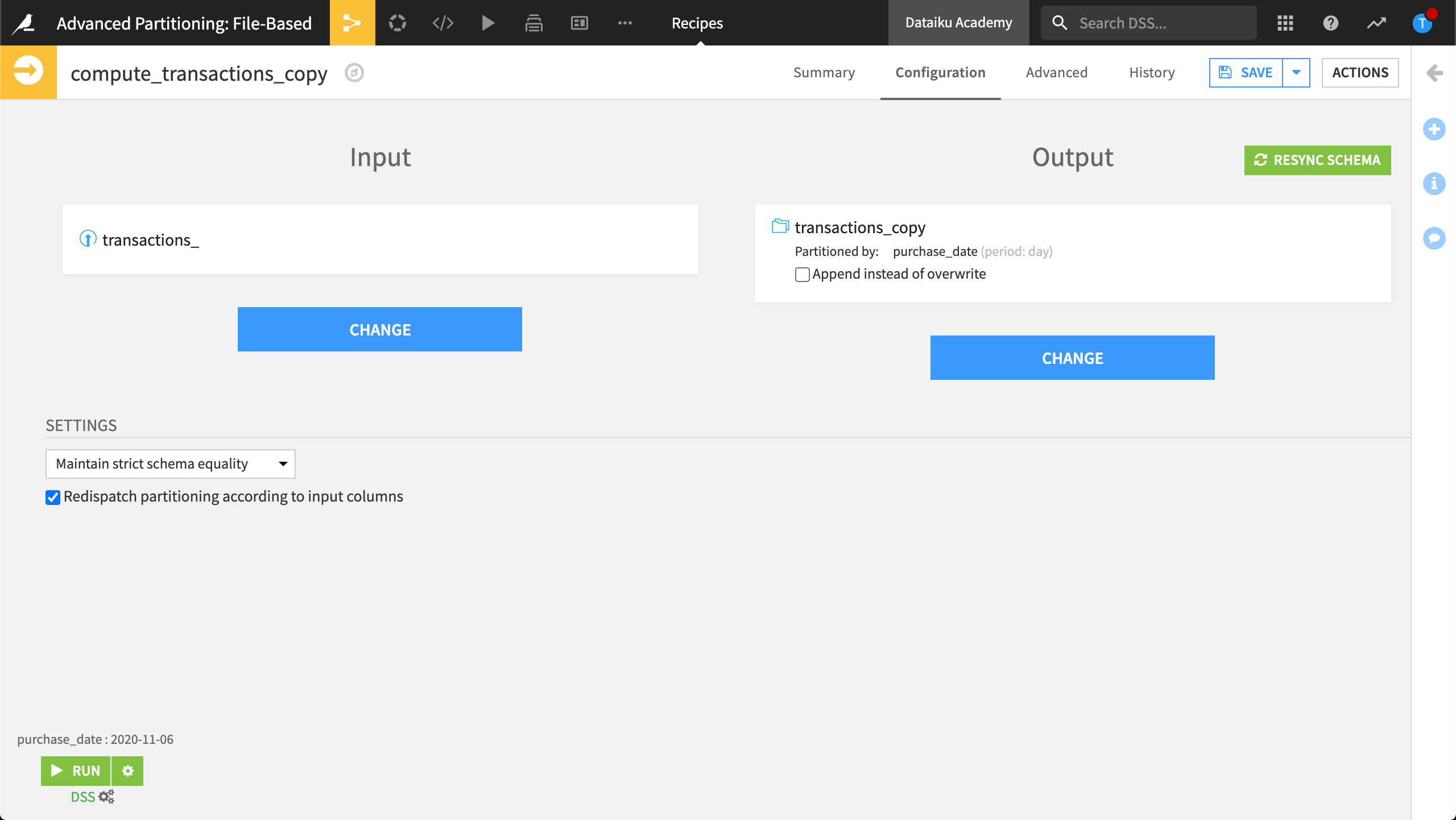
To define how we want to partition our dataset, we must first configure the Sync recipe.

1. Once again, open the Sync recipe that was used to generate transactions_copy.

2. Click Redispatch partitioning according to input columns, then click Save.

   Dataiku warns that a schema update is required. This is because redispatching removes the purchase_date column when our dataset is stored on a file system.

3. Click Update Schema to accept the schema change.

   

   Note

   The current date displays above the Run button. The Recipe run option requires you to define a partition to build. The value you specify does not impact the output, it is simply a “dummy” value. The Partition Redispatch feature computes all possible partitions within the data, building all partitions at once, regardless of the value you specify.

4. Click Run to build the dataset.

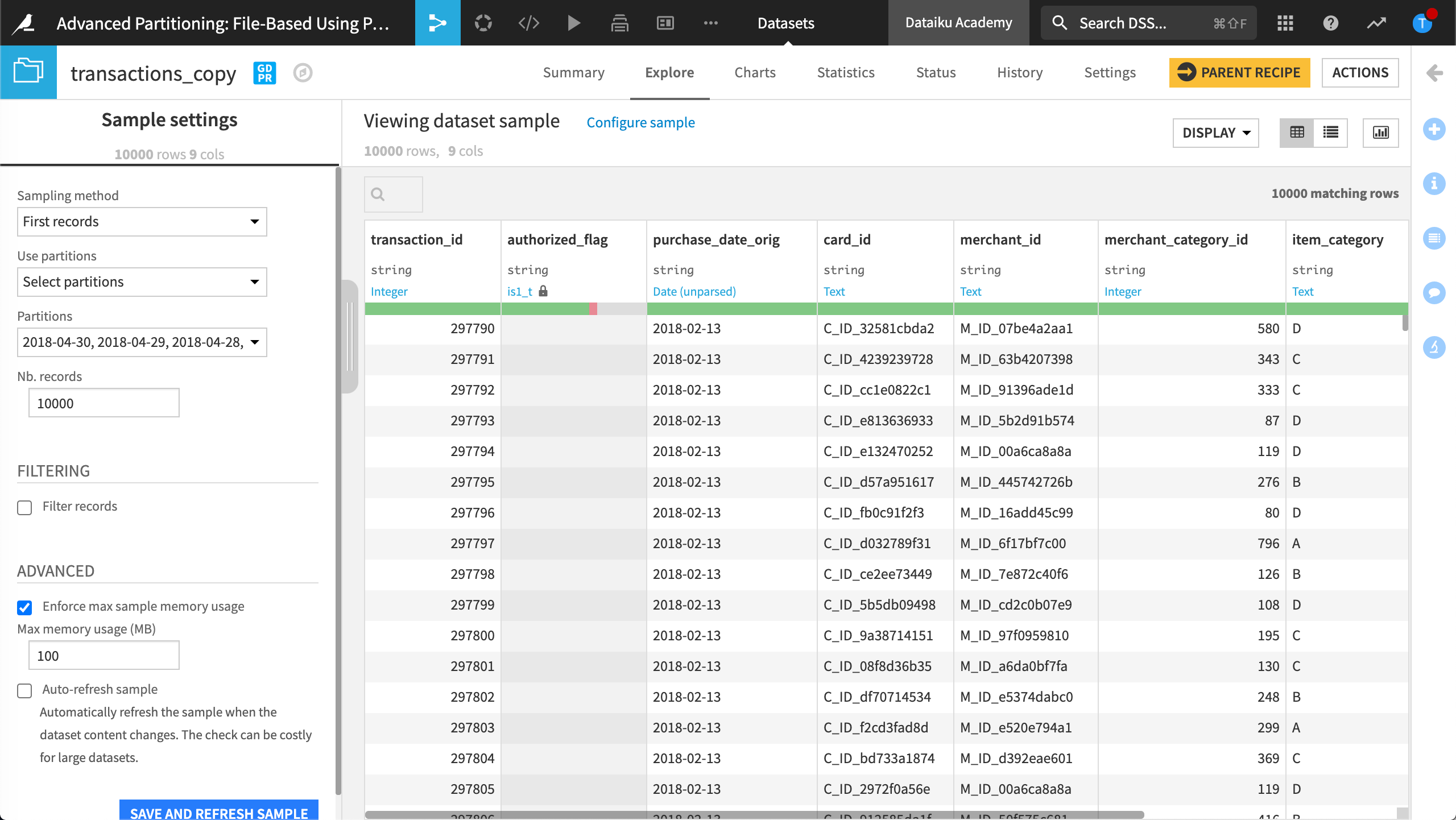
5. Explore the resulting output dataset, transactions_copy.

The output dataset seems unremarkable, except the purchase_date column is no longer visible. This is expected because in file-based partitioning, the partition is in the file name, not the data.

To view the new partitions:

1. Click Configure sample.

2. In Sample Settings, under Use partitions, choose Select partitions.

3. Retrieve the list of partitions, then select all partitions.

4. Click Save and Refresh Sample.

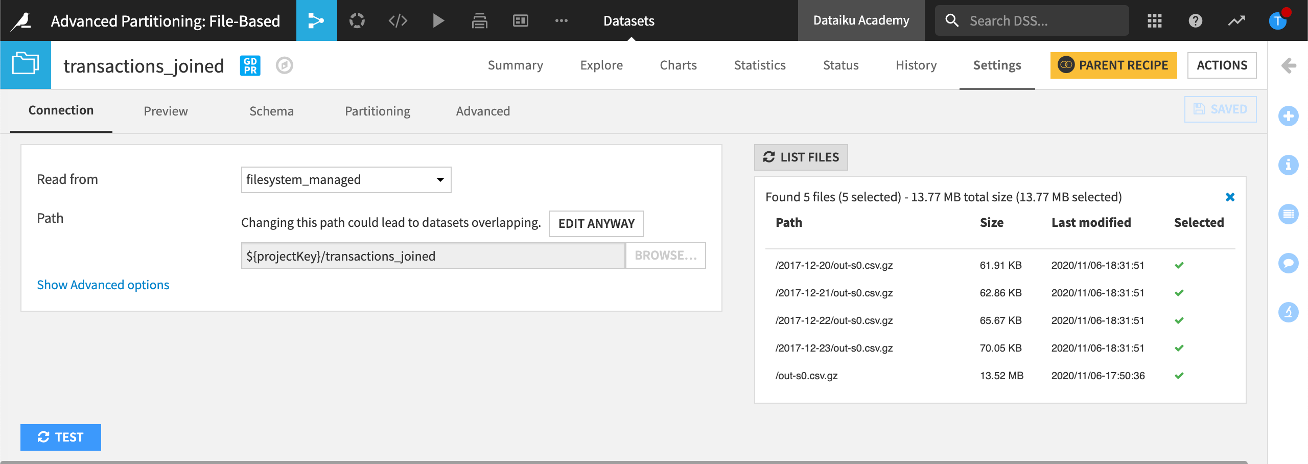
To see how Dataiku stores the data on the filesystem connection once the file-based partitioning is enabled, you can view Settings, and then List Files.

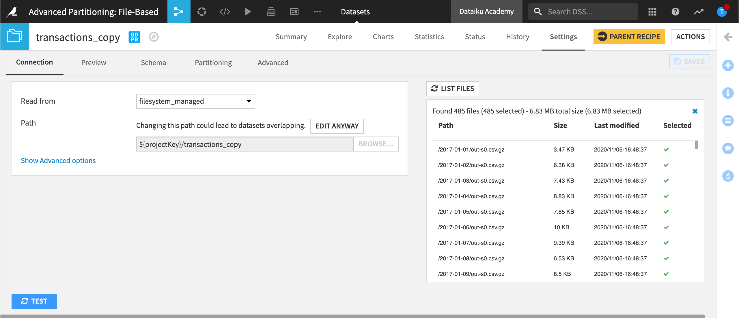
In this example, Dataiku found 485 files. In other words, this dataset is made up of 485 partitions.

Propagate the time-based partition dimension across the Flow

Now that our first dataset is partitioned, we can propagate the partitioning dimension across the Flow.

Build the transactions_joined dataset

To build the transactions_joined dataset, do the following, updating the schema when prompted:

1. Return to the Flow.

2. Open and run the Sync recipe that was used to create merchant_info_copy.

3. Open and run the Sync recipe that was used to create cardholder_info_copy.

4. Open and run the Join recipe that was used to create transactions_joined.

Note

The transactions_joined dataset contains duplicate records after partitioning it.

Partition the transactions_joined dataset

Partition transactions_joined and identify the partition dependence using the following steps:

1. Open the transactions_joined dataset.

2. View Settings > Partitioning.

3. Click Activate Partitioning.

4. Click Add Time Dimension.

5. Name the Dimension purchase_date, and set the Period to Day.

6. Set the Pattern to %Y-%M-%D/.*.

7. Click Save and click Confirm to confirm that dependencies with this dataset will be changed.

Note

Clicking List Partitions results in zero detected partitions. This is because even though we have configured the partitioning dimension, we have not yet built any partitions in the dataset.

Your Flow now contains two layered icons: transactions_copy and transactions_joined. Both datasets are partitioned using the purchase_date dimension.

Identify the partition dependencies

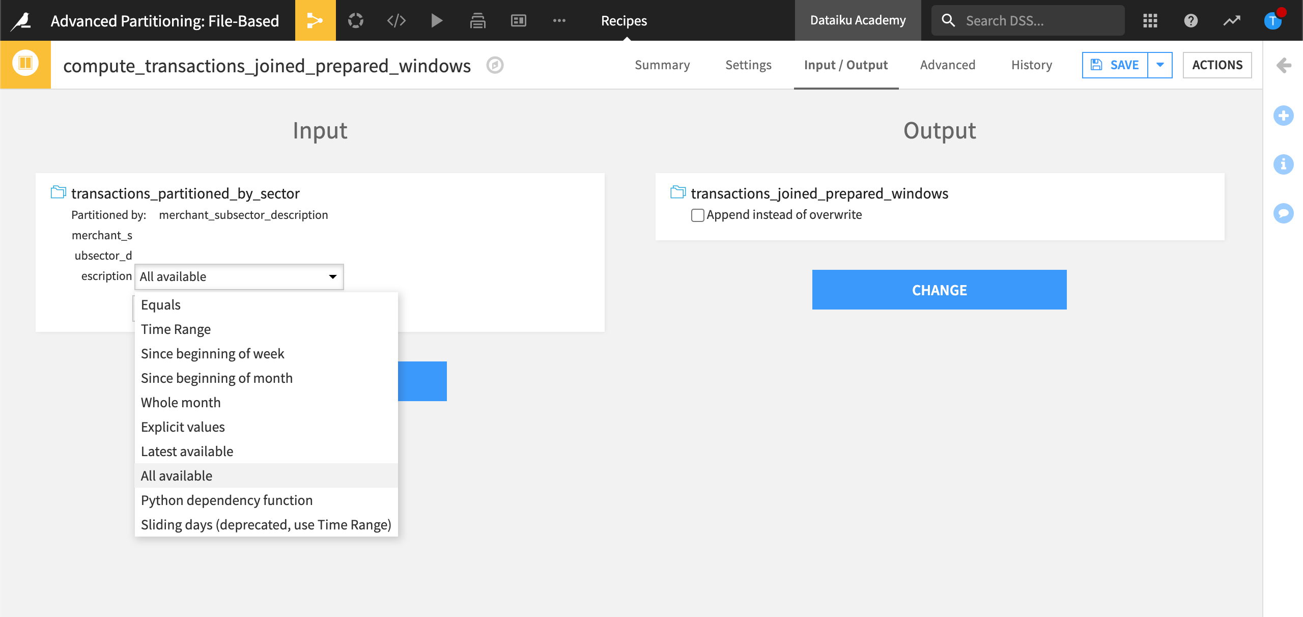
Now we must identify which partition dependency function type (e.g., ‘All available’, ‘Equals’, ‘Time Range’, etc.) we want to map between the two datasets, transactions_copy and transactions_joined. We can also specify a target identifier, such as a specific calendar date.

To do this, modify the Join recipe:

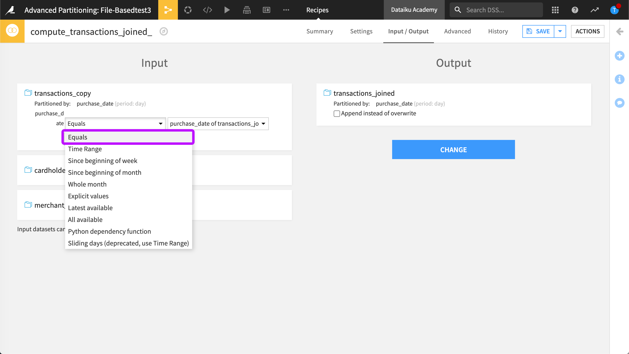
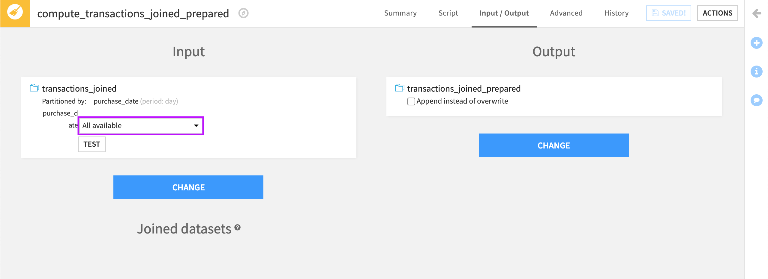
1. Open the Join recipe and view the Input / Output tab.

   By default, Dataiku sets the partition mapping so that the output dataset is built, or partitioned, using all available partitions in the input dataset.

   To optimize the Flow, we only want to target the specific partitions where we are asking the recipe to perform computations.

2. In the partitions mapping choose Equals as the partition dependency function type.

   

3. View the Settings tab.

4. Click the Recipe run options icon next the Run button, and select Specify explicitly.

5. Type the value, 2017-12-20,2017-12-21,2017-12-22,2017-12-23, then click OK.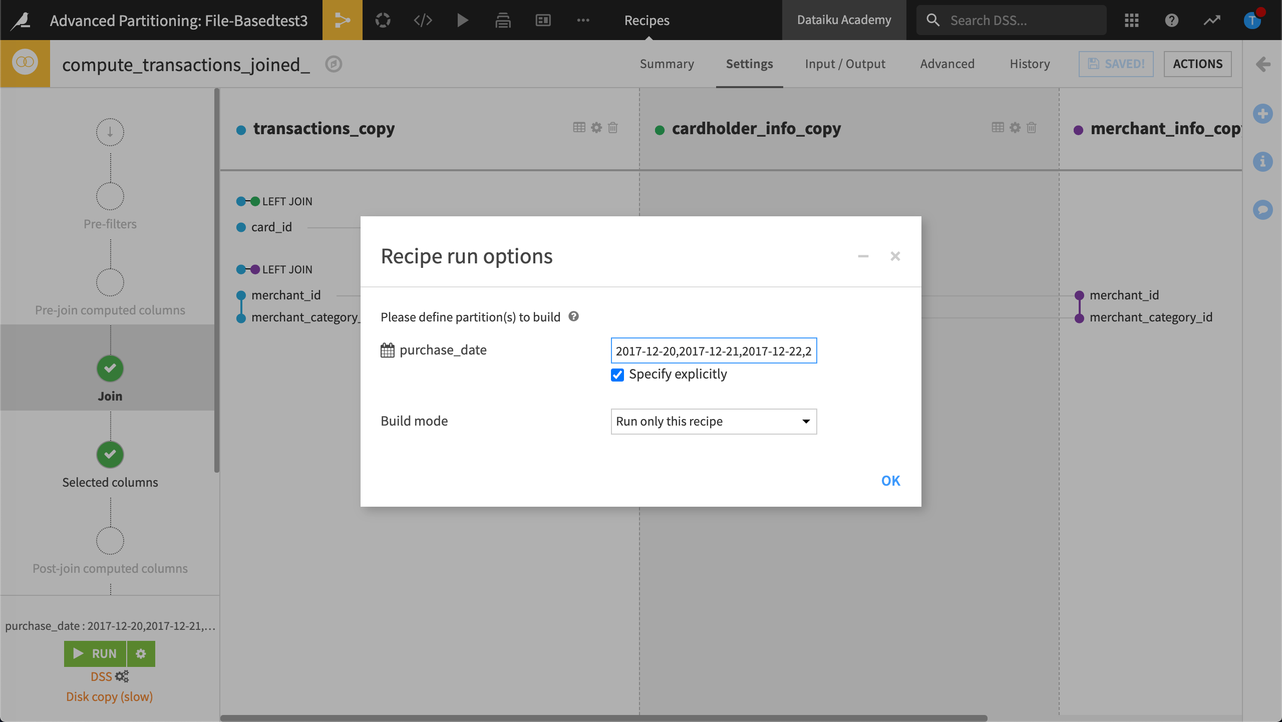

   

6. Without running the recipe, click Save.

   The recipe is now configured to compute the Join only on the rows belonging to the dates between “2017-12-20” and “2017-12-23”.

7. Do not run the recipe yet.

Run a partitioned job

Let’s run a partitioned job.

1. Return to the Flow.

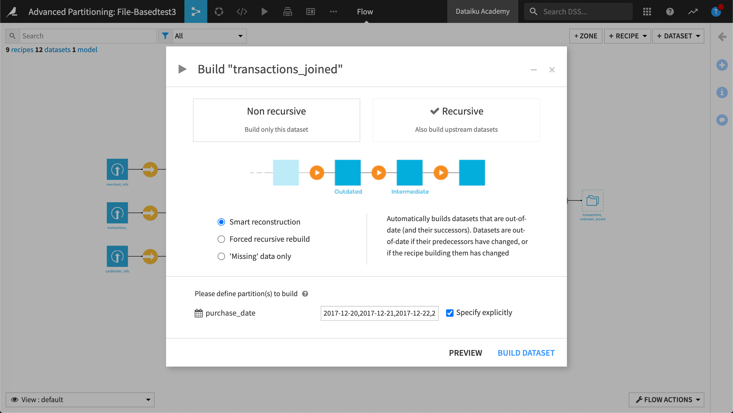
2. Right-click transactions_joined and select Build from the menu.

3. Choose a Recursive build.

4. Select Smart reconstruction.

5. Click Build Dataset.

   

6. While the dataset is building, view the most recent Job.

   

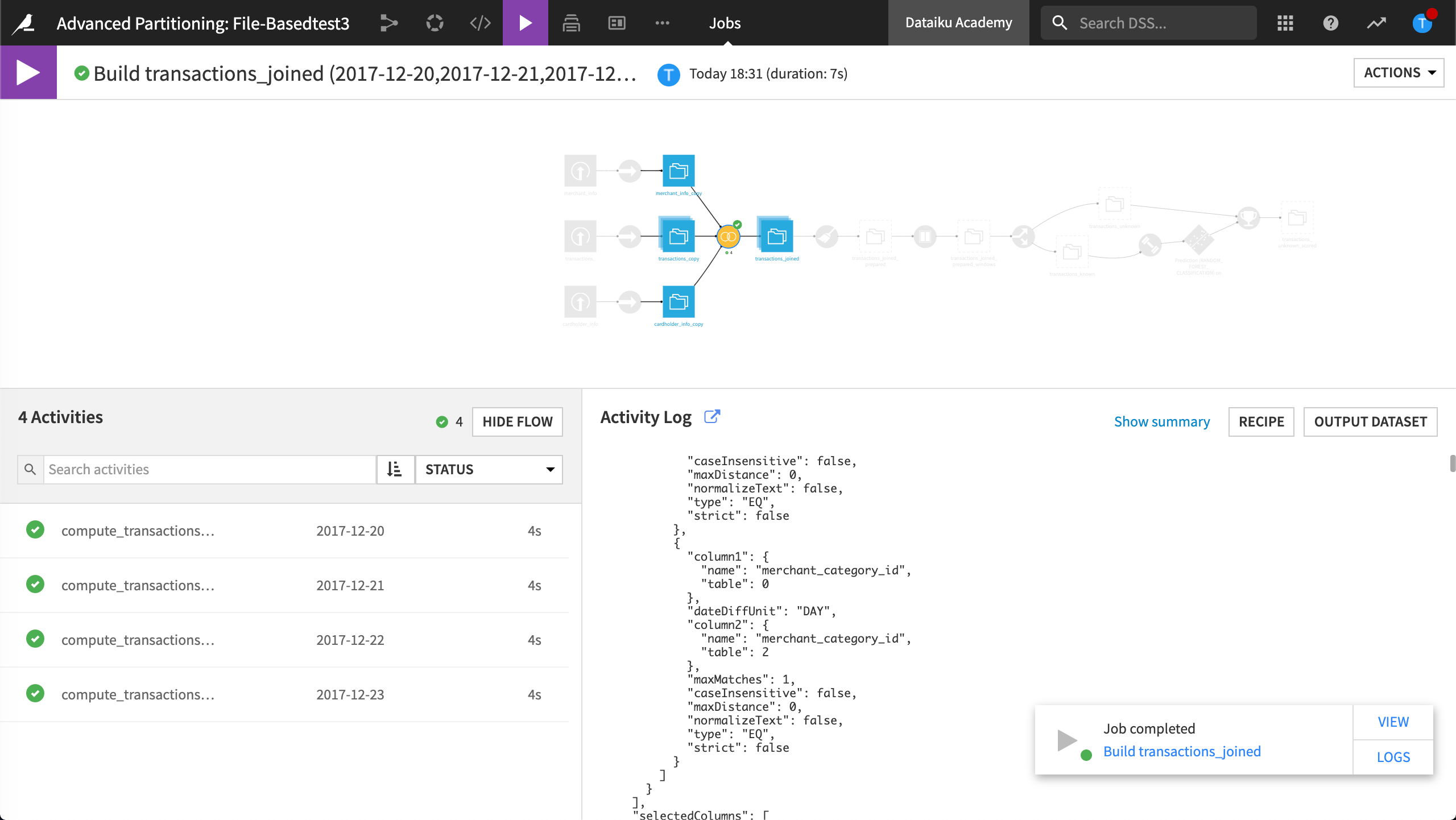
   The most recent job shows which dataset’s partitions are being built. In Activities you can see the requested partitions.

7. Return to the Flow.

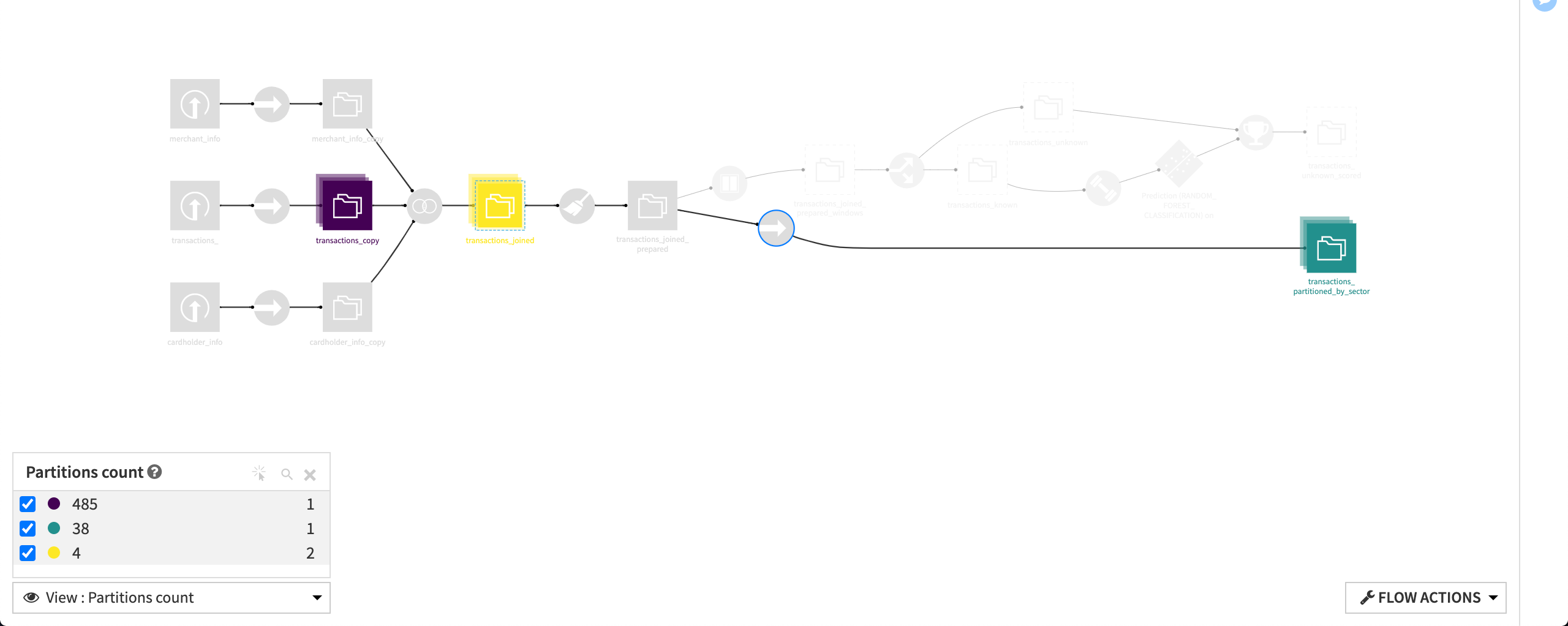
8. From the Flow View, select to visualize the Partitions count.

   

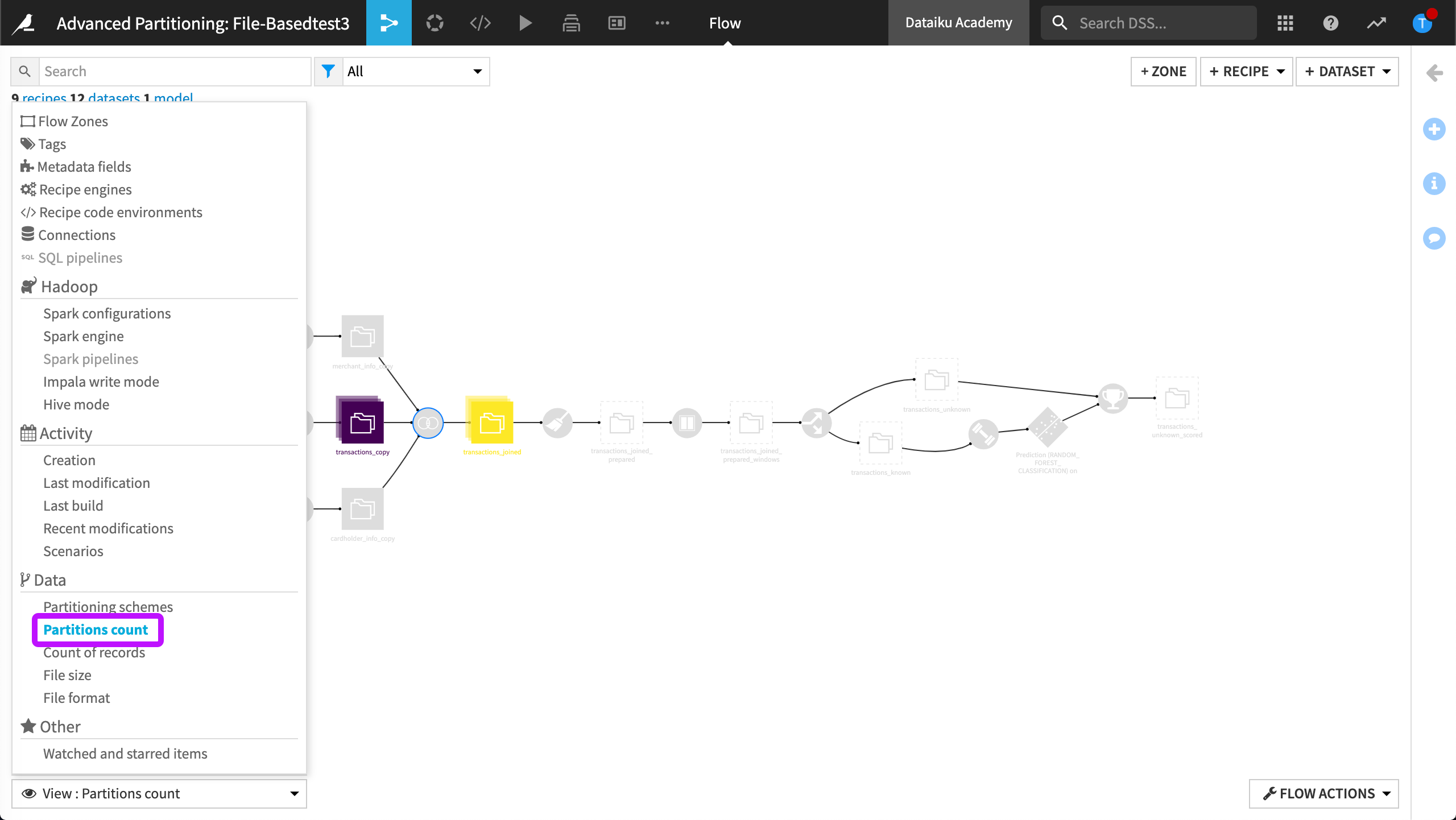
   Using this view, we can see that the job is completed.

9. Close the Partitions count view to restore the default view.

Stop the partitioning and retrieve the partitioning dimension information

We will now stop the partitioning of our purchase_date dimension and create a non-partitioned dataset. To do this, Dataiku uses a “partition collection” mechanism during runtime. This mechanism is triggered by the partition dependency function type, “All available”.

This process is referred to as partition collecting. Partition collecting can be thought of as the reverse of partition redispatching.

We will also retrieve the partitioning dimension information.

Background

Recall that we partitioned the dataset, transactions_copy by “day” using the purchase_date dimension. These dimensions did not already exist in their own file paths, so we used the Partition Redispatch feature to create the partitions. This had the impact of creating separate files, as evidenced when we listed the files.

We were then no longer able to view the purchase date column that was used to partition the dataset when we explored the dataset.

Note

Starting with Dataiku 8.0.1, you can use the “Enrich record with context information” processor to create a new column, with a new name, to restore information that was used to partition a dataset. In this way, you would not have to keep a duplicate purchase_date column in the transactions dataset.

Later, we edited the Join recipe to define which rows we wanted by typing the value, 2017-12-20,2017-12-21,2017-12-22,2017-12-23. This had the effect of computing the Join only on the rows belonging to the dates between “2017-12-20” and “2017-12-23”.

Then we ran a partitioned job and were able to visualize our partitions in the Flow.

Now, we will parse the purchase_date_orig column, which is a duplicate of the original purchase date column, and extract the date components. We’ll also compute the number of days the card has been active. The reason we want to do this is because per our business objectives, we want to be able to compute features for a machine learning model.

This is a multi-step process.

Parse the original purchase date and extract date components

To parse the original purchase date and use it to extract date components, we’ll use a Prepare recipe.

1. Open the compute_transactions_joined_prepared Prepare recipe.

2. Review the Date formatting group.

   The Date formatting group contains the steps needed to parse dates, extract date components, create a new column, purchase_weekend, and compute the time difference between card_first_active_month_parsed and purchase_date_parsed.

3. Run the recipe.

   Dataiku builds transactions_joined_prepared.

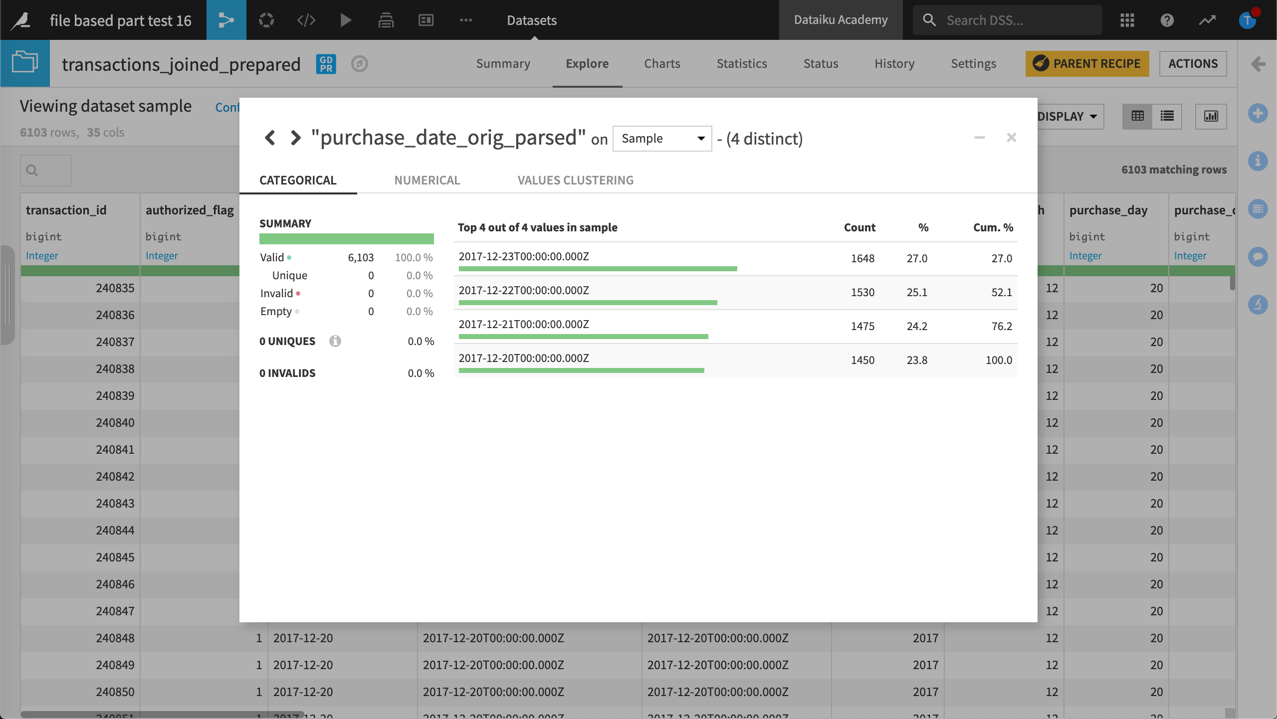
4. Explore the output dataset and analyze the purchase_date_orig_parsed column to see that it contains the dates resulting from the computation that was configured in the Join recipe.

Build a discrete-based partitioned dataset

Recall from the business objectives that we want to be able to predict whether or not a transaction is fraudulent based on the transaction subsector (e.g., insurance, travel, and gas) and the purchase date. This is discrete information.

To meet this objective, we need to partition the Flow with a discrete dimension. This requires a Sync recipe.

1. Select the transactions_joined_prepared dataset and add a Sync recipe.

2. Name the output dataset transactions_partitioned_by_sector.

   The Partitioning option should be set to Not partitioned.

3. Click Create Recipe.

4. Run the recipe and explore transactions_partitioned_by_sector.

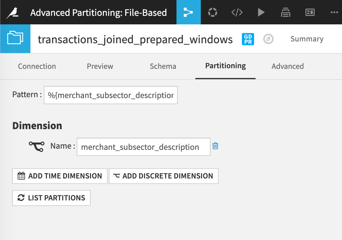
5. View the Settings tab and click the Partitioning subtab.

6. Click Activate Partitioning then Add Discrete Dimension.

7. Name the Dimension merchant_subsector_description to match the name of the column in the dataset.

8. Click the pattern in Click to insert in pattern.

   

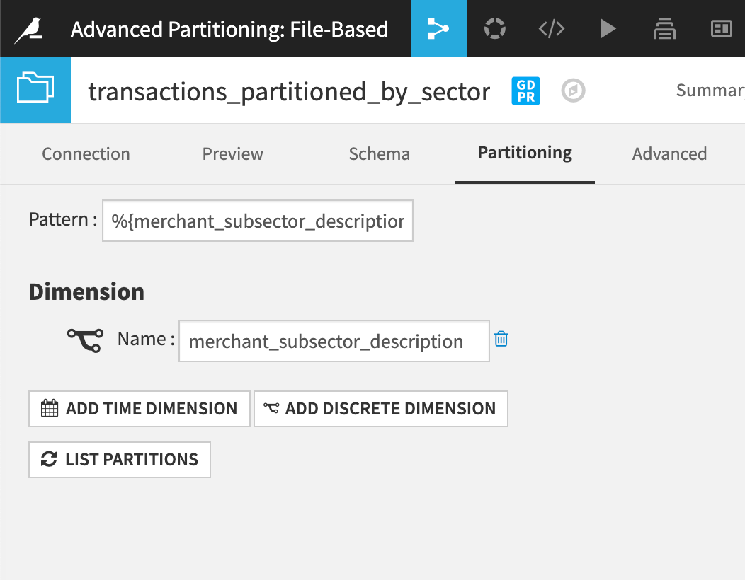
   The partitioning configuration is complete.

9. Click Save and return to the Flow.

Your Flow now looks like this:

Modify the Sync recipe

Next, we’ll modify the Sync recipe that generates transactions_partitioned_by_sector.

1. Open the Sync recipe and enable the partition redispatch by selecting the Redispatch partitioning according to input columns option.

   The Run button is disabled because we have not yet defined a partition for this job.

2. Click the Recipe run options icon next the Run button.

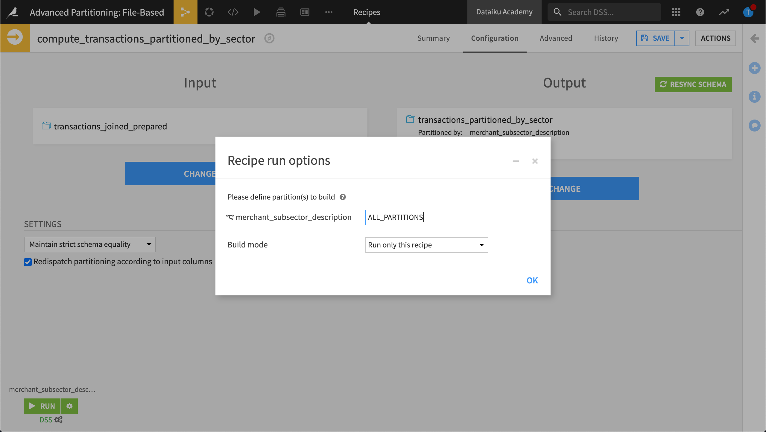
Partition redispatch computes all existing partitions regardless of what value we specify here. But, we’ll use “All partitions”.

1. Type the value, ALL_PARTITIONS, then click OK.

2. Click Save and accept the schema change.

3. Run the recipe and return to the Flow.

4. From the Flow View, select to visualize the Partitions count.

   

   The Partitions count displays a count of 38 partitions in the dataset transactions_partitioned_by_sector.

5. Close the Partitions count view to restore the default view.

Adapt the Flow to the discrete partitioning

In this section, we will change the Window recipe’s input so that it is mapped to transactions_partitioned_by_sector.

1. Open the Window recipe.

2. In the Input / Output tab, Change the input dataset, replacing transactions_joined_prepared with transactions_partitioned_by_sector.

   Note that the partition dependency is set to All available. We will change this later.

   

3. Save the recipe, updating the schema.

4. Return to the Flow.

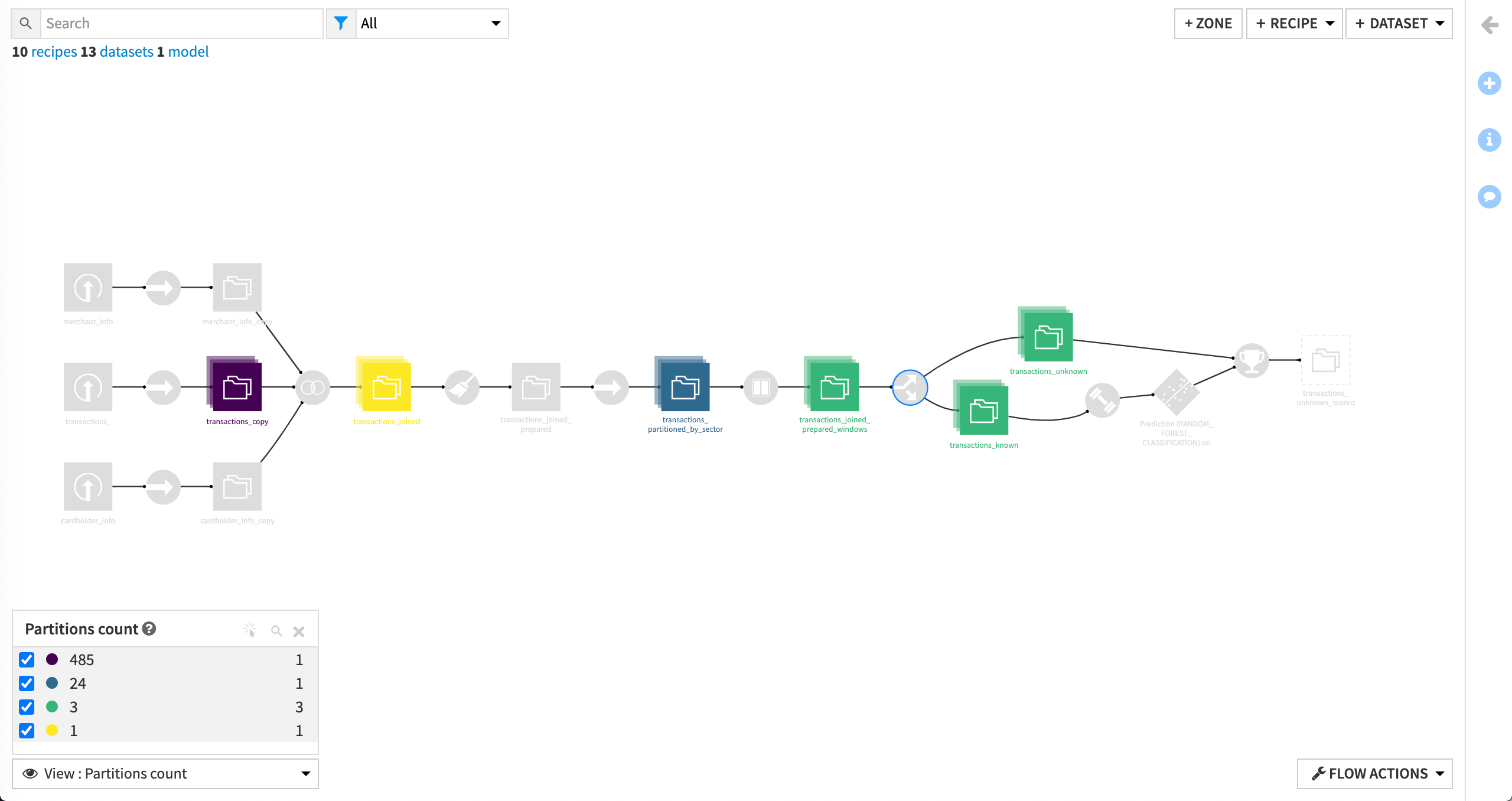
5. From the Flow View, select to visualize the Partitions count once again.

The Flow contains 485 time-based partitions and 38 discrete partitions. We reduced the number of time-based partitions to 4 partitions when we configured the Join recipe to compute only on the rows belonging to the dates between “2017-12-20” and “2017-12-23”.

If we ever need more data we can simply reconfigure the Join recipe to ask for additional “date” partitions.

Before we propagate the discrete partitioning dimension through the Flow, we will analyze the transactions_partitioned_by_sector dataset.

Analyze the partitioned dataset

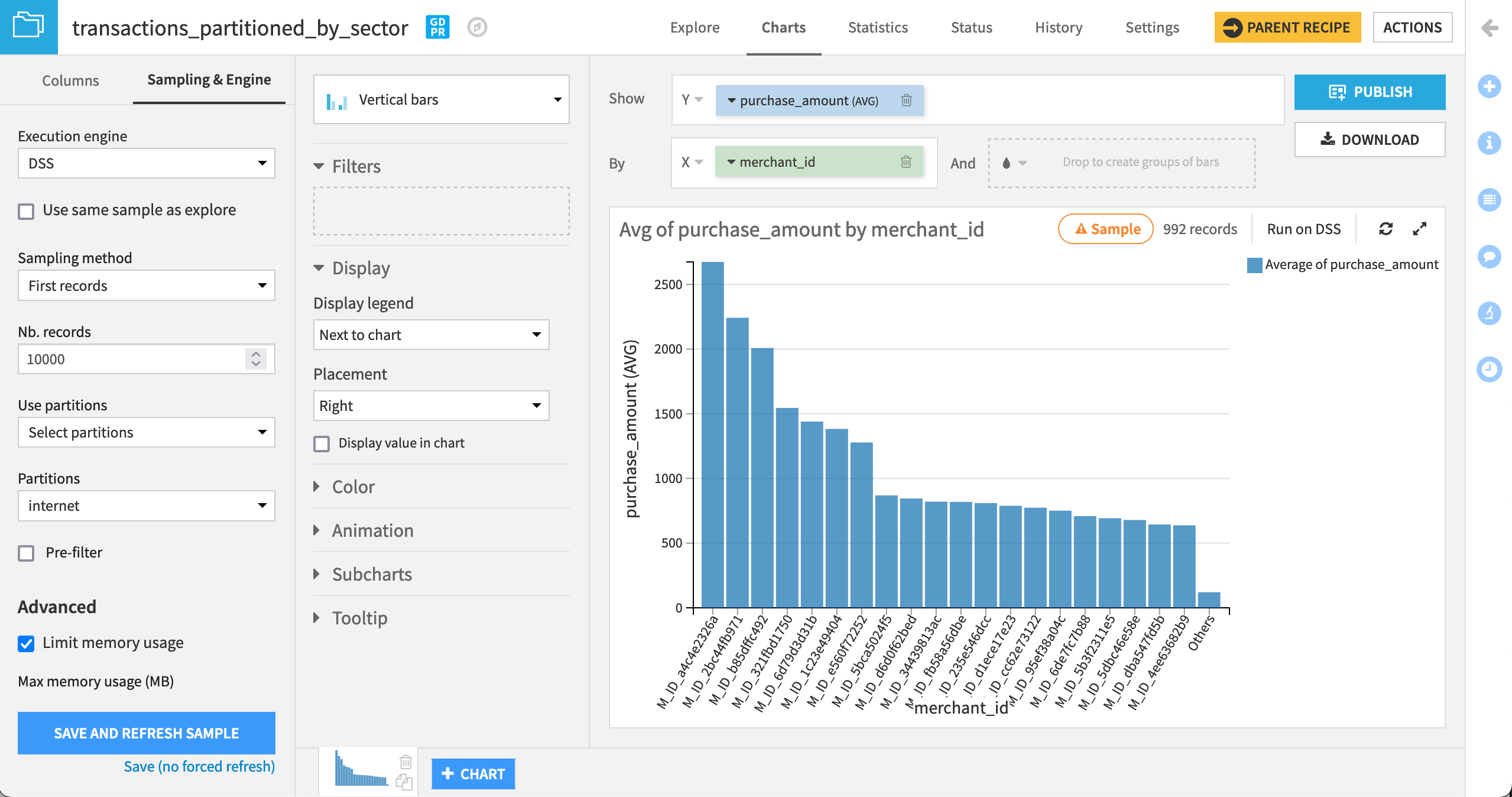
Analyze the purchase amount earned by each merchant.

To do this:

1. In the Flow, explore transactions_partitioned_by_sector and visit the Charts tab.

2. Set the x-axis to merchant_id dimension and the y-axis to purchase_amount (AVG).

Analyze this information by the “internet” subsector. To do this, you can use the “internet” partition.

1. Click the Sampling & Engine tab at the top.

2. Deselect the Use same sample as explore option.

3. In Use partitions, choose to Select partitions.

4. Click the Retrieve List icon, then choose the internet partition.

5. Click Save and Refresh Sample to generate the chart.

6. Sort merchant_id by Average of purchase_amount, descending.

Dataiku displays the merchant gains on products belonging to the internet partition.

We can also perform other bivariate analyses in order to analyze the purchase amount.

1. Navigate to the Statistics tab.

2. Click +Create Your First Worksheet.

3. Select Bivariate Analysis.

4. Configure the card so that card_age is a Factor and purchase_amount is a Response.

5. Select Histogram and Box Plot as options.

6. Click Create Card.

   

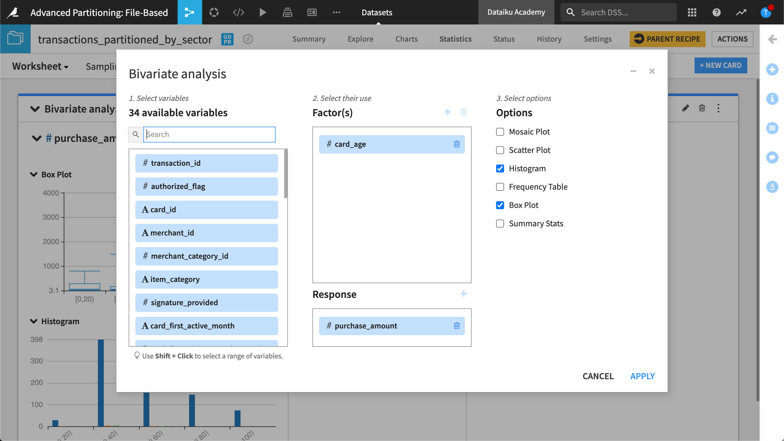
   Dataiku displays the distribution by state.

7. Since we only want the internet partition, tune the Sampling and filtering option.

Dataiku displays the bivariate analysis for the purchases based on the internet partition.

Propagate the discrete partitioning through the Flow

Now you can apply what you’ve learned to propagate the discrete partitioning through the Flow. To do this, follow the same process you used to propagate the time-based partitioning through the Flow.

Step 1. Partition the output datasets

1. Run the Window recipe.

2. Partition transactions_joined_prepared_windows by merchant_subsector_description dimension.

   

3. Right-click the Split recipe and select to Build Flow outputs reachable from here.

4. Partition transactions_known by merchant_subsector_description dimension.

5. Partition transactions_unknown by merchant_subsector_description dimension.

6. Partition transactions_unknown_scored by merchant_subsector_description dimension.

Step 2. Modify the recipe mappings

In this section, we will update the partition dependency mappings and define specific partitions to build in the Window and Split recipes.

We will use “Equals” as the partition dependency function and gas/internet/insurance as the specific partitions to build.

1. Open the Window recipe and go to the Input / Output tab.

2. In the partitions mapping, choose Equals as the partition dependency function.

3. View the Settings tab.

4. Click the Recipe run options icon next the Run button.

5. Type the value, gas/internet/insurance to define the partitions to build, then click OK.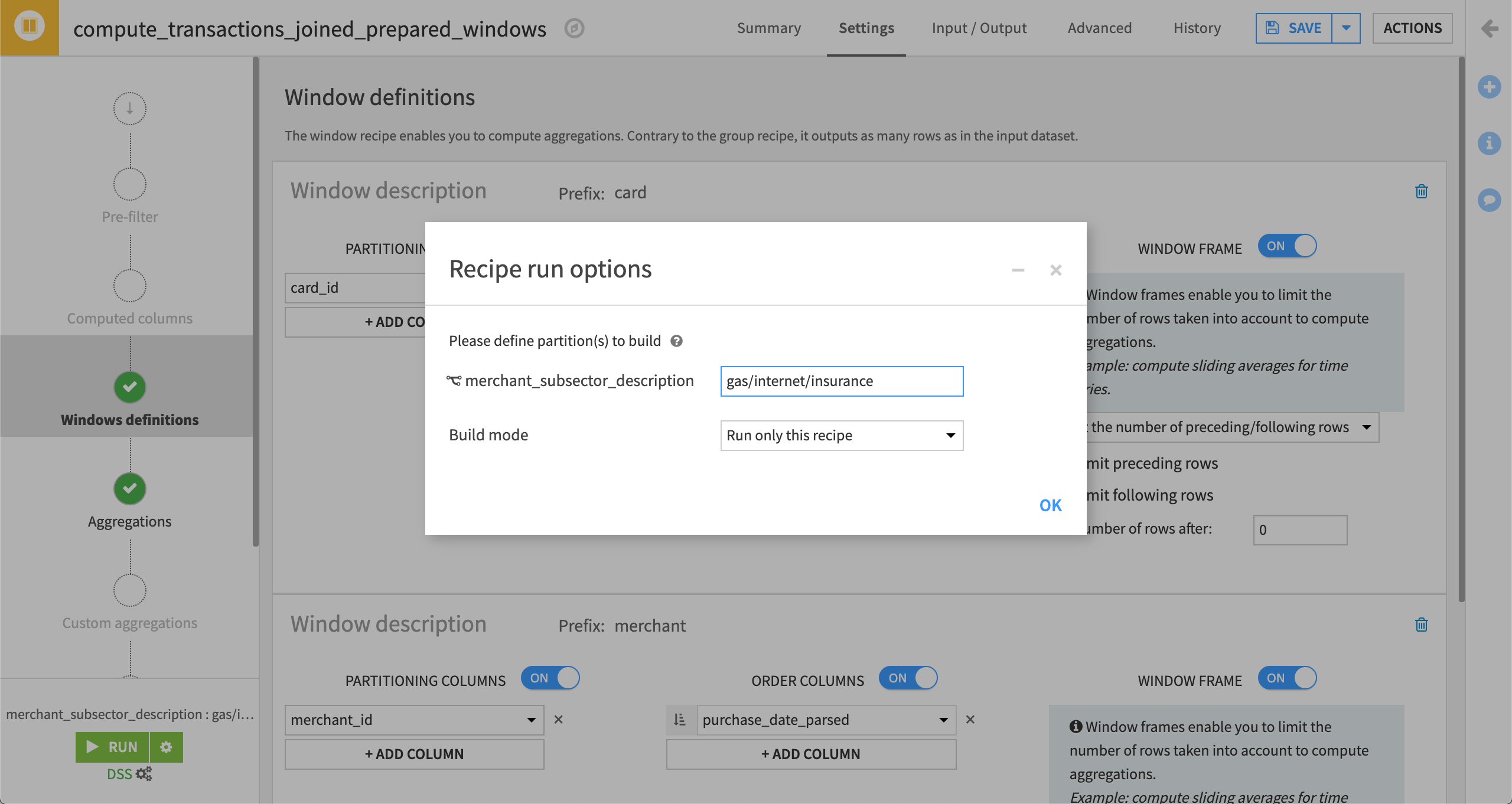

   

6. Save and Run the recipe.

Finally, let’s update the Split recipe in a similar manner.

1. Open the Split recipe and go to the Input / Output tab.

2. In the partitions mapping, choose Equals as the partition dependency function.

3. View the Settings tab.

4. Click the Recipe run options icon next the Run button.

5. Ensure that gas/internet/insurance are the defined partitions to build, then click OK.

6. Save and Run the recipe, updating the schema.

The Flow now looks like this:

Congratulations! You have completed the tutorial.

What’s next?

Now that the datasets in the Flow are partitioned, you could train the partitioned machine learning model to detect fraud by subsector.

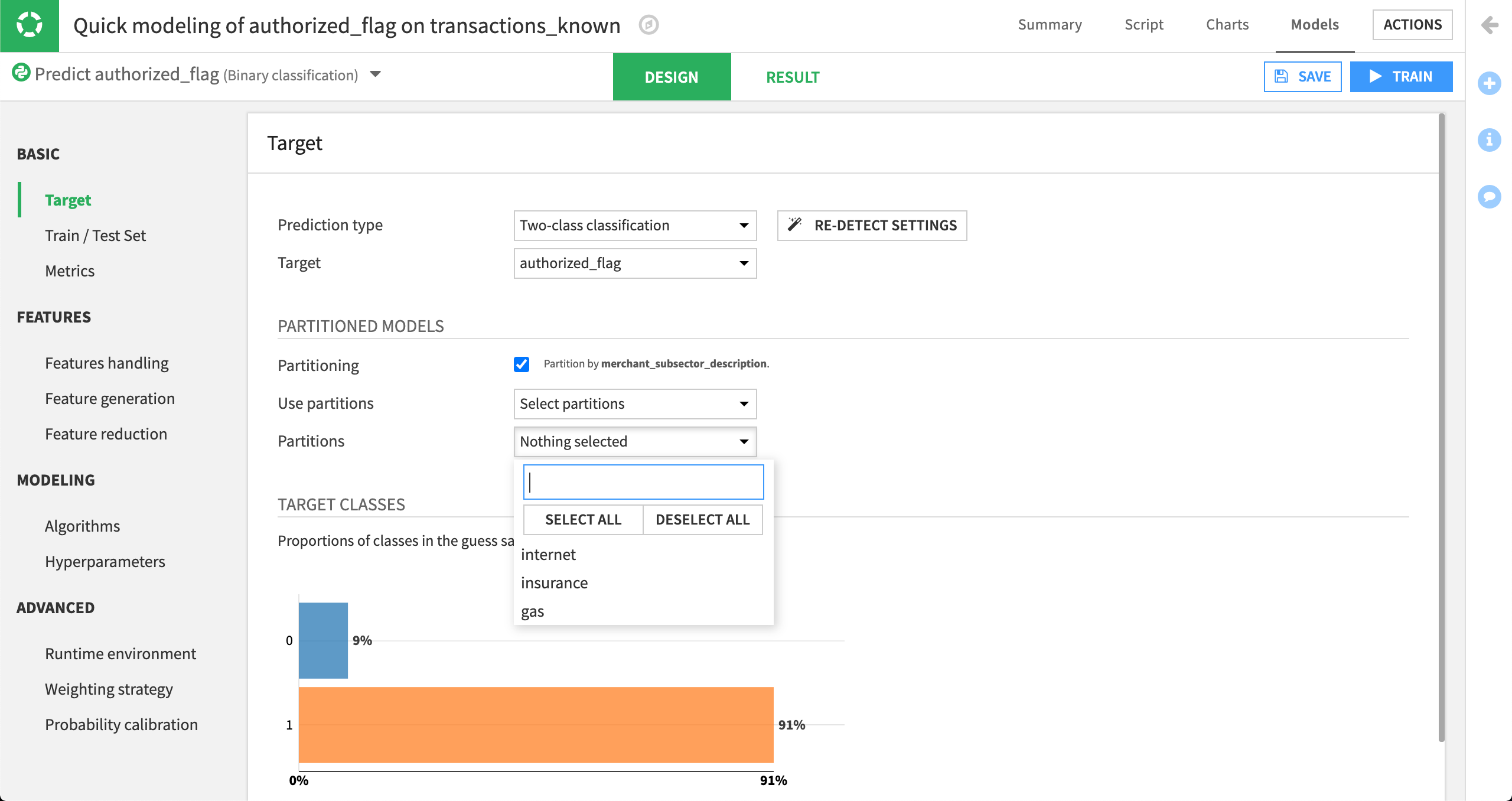
Visit the course, Partitioned Models, to learn more about training a machine learning model on the partitions of a dataset.