
Concept | Time series interval extraction#
An overview of time series interval extraction#
When working with time series data, we’re sometimes interested in data that lie within specified boundary values, and finding the corresponding time segments for this data.
We’ll tackle this topic in three parts:
The motivation for interval extraction with time series data.
The mechanics behind the Interval Extraction recipe in the time series preparation plugin.
Demo: how to use the recipe in Dataiku.

The motivation for interval extraction of time series#
Watch the video or read the summary below.

Imagine a factory where the production line follows a normal distribution. Every minute, the line produces, on average, mu items with some standard deviation sigma.
Suppose we want to flag time intervals during which the factory produced more than three standard deviations greater than or less than the average. We could then investigate the conditions associated with these anomalies. How could we identify these time intervals with our existing tools in Dataiku?

To build up to this use case, let’s return to our familiar example of t-shirt revenue, plotted on the y-axis, across time, plotted on the x-axis. Imagine we want to identify intervals of typical days, that is, days when the revenue lies between $25,000 and $35,000.
For each row of the data, we ask one simple question. Does the value lie within our threshold range?

To achieve this, you could use a Filter recipe or a Filter processor in a Prepare recipe, for example. But with time series, we sometimes want to attach conditions in addition to setting an upper and lower bound.

In this article, we’ll discuss three advantages that the Interval Extraction recipe in the Time Series Preparation plugin offers above the basic kind of filtering.
For example, we may want to:
Keep track of retained intervals.
Define an acceptable deviation period.
Define a minimal segment deviation.

Intervals#
Remember that time series aren’t made of independent observations. Rather, these observations are dependent on time. This means that the valid intervals — the time periods containing observations that lie between the upper and lower bound — represent valuable information.

For this reason, we often want to keep track of those valid intervals by using a different ID for each interval as we move along the time series from start to finish. Once we have the intervals recorded in our dataset, we can define new features to use for modeling or for further analysis.
For example, we can use a Window recipe to calculate the average length of an interval or the elapsed time since the previous interval.

Acceptable deviation#
Setting an acceptable deviation can be particularly useful in cases where volatility exists in our time series, and we want our time intervals to retain brief deviations from the threshold range, while excluding longer deviations.

In our example, consider that the point for July 3rd is out of the threshold range. However, the previous timestamp is in the threshold range. And the next timestamp is also back in the threshold range. The time series skipped out of range for just one day.

By setting an acceptable deviation of one day, we would absorb the point for July 3rd, as well as the point for July 1st, into one single time interval with its neighbors.

However, the points for July 5th and 6th are outside the threshold range for a time period that’s longer than the acceptable deviation. We would need an acceptable deviation of at least two days if we wanted to include these points in an interval ID.

Minimal segment duration#
Finally, let’s see how to define a minimal segment duration for retained time intervals.
While the acceptable deviation parameter gives us the flexibility to expand a valid time interval, the minimal segment duration parameter does just the opposite by imposing a minimum requirement on the duration of a valid interval.
In the short interval shown in the center below, all values lie within the threshold range. But perhaps, we require all intervals to be at least 7 days long. To enforce this requirement, we could set a minimal segment duration of 7 days, and thereby prevent intervals shorter than 7 days from being assigned an interval ID.

Let’s see this in the table where the acceptable deviation and the minimal segment duration are both set to 0 days.
The first two intervals (July 2nd and July 4th) include only one valid timestamp. That makes their segment duration, or the difference between the first and the last valid timestamp, equal to 0 days.
If the minimal segment duration is 0, these single timestamps will remain separate interval IDs.

However, if we increase the minimal segment duration to one day, now these intervals are too short. They fail this requirement, and so Dataiku won’t assign them to an interval.

The mechanics of the interval extraction recipe#
Watch the video or read the summary below.
Now that you have a sense of the recipe’s intuition, let’s dive into the recipe’s mechanics!

We’ll continue with the same example time series and the same threshold range used in the first part of the article.

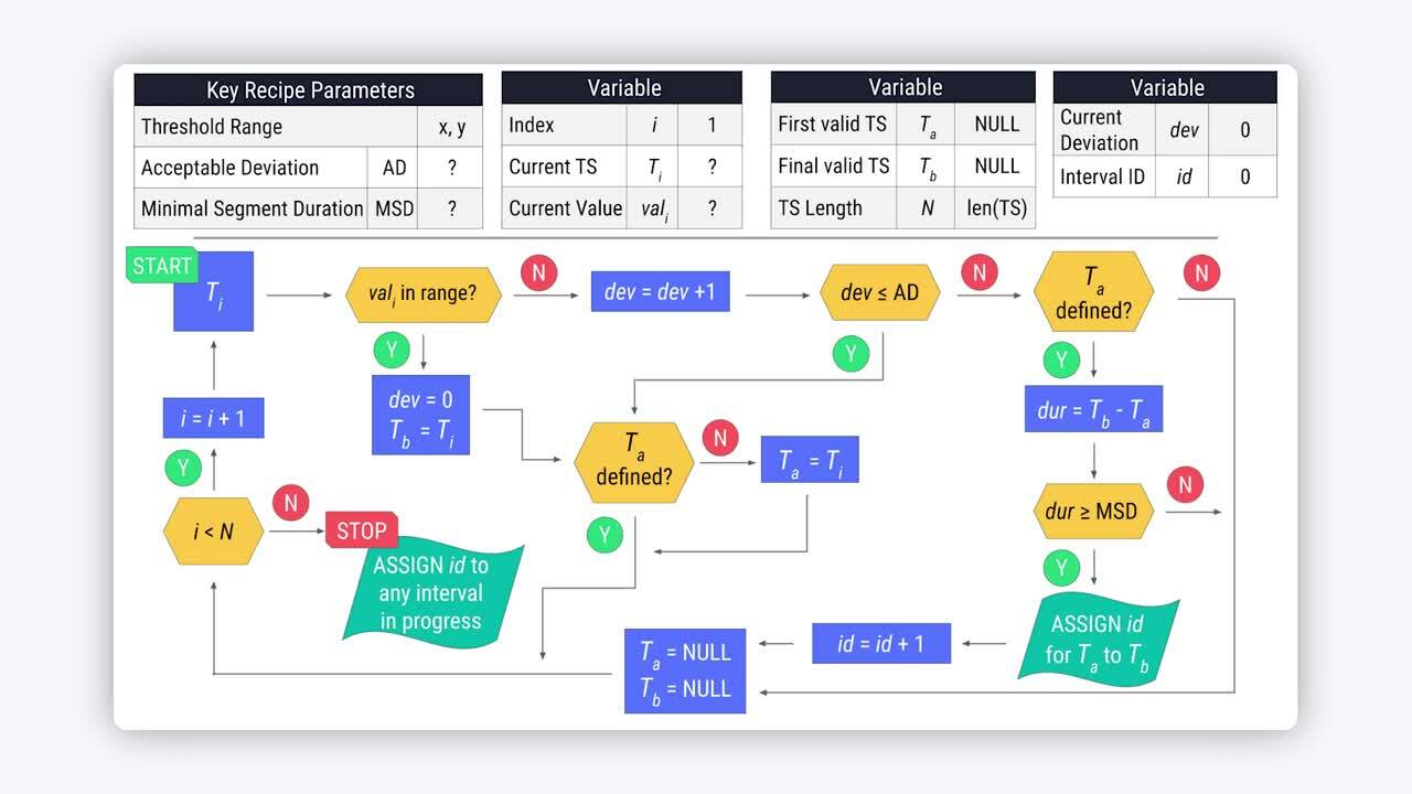
This flowchart captures how the Interval Extraction recipe functions.

Recipe parameters and variables#
Let’s start with the key recipe parameters. The threshold range set by the user is 25 to 35, and, for this example, we’ll set the acceptable deviation and the minimal segment duration to one day.
As we walk along the time series row by row, we’ll need to keep track of a few different variables.
Let \(i\) represent an index starting from 1.
As we increment \(i\) row by row, \(T_i\) represents the current timestamp. So, if \(i\) is 1, \(T_i\) or \(T_1\), is the first timestamp.
In the same row as the current timestamp is the current value, or \(val_i\).
Next, we’ll have to keep track of the timestamps marking the beginning and end of a valid interval.
That is \(T_a\) and \(T_b\).
These values are both initially NULL because we don’t yet have a candidate for a valid interval.
We’ll also need to know the total number of timestamps in the series, to use in the stopping criterion for the process described in the flowchart.
We’ll call it \(N\).
We also have to maintain a counter for the current deviation from the threshold range.
We’ll call it \(dev\) and initialize it to 0.
Should any number of timestamps meet the conditions set by the segment parameters, the recipe will assign interval IDs using the \(id\) variable.
The recipe starts assigning IDs from 0, so we’ll initialize the variable \(id\) to 0.
Recipe results#
Mastering this recipe takes some practice. Here are the results for the example time series above using three different sets of segment parameters.
Acceptable deviation: 0 Days; Minimal segment duration: 0 Days#

Acceptable deviation: 0 Days; Minimal segment duration: 1 Day#

Acceptable deviation: 1 Day; Minimal segment duration: 1 Day#

Be sure to try out a few examples on your own with different segment parameters to make sure you have got the hang of it!
Using the interval extraction recipe in Dataiku#
Watch the video or read the summary below.
After having explored the motivation and mechanics of the Interval Extraction recipe from the Time Series Preparation plugin, let’s finally test out how it works in Dataiku.

As shown in Concept | Time series resampling, we used the Resampling recipe to equally space and interpolate the wide version of the orders data.
Having multiple independent time series (one for each product category), we’ll have to work with the data in long format to apply the Interval Extraction recipe.

It’s not required, but it’s often advisable to first resample the data to make sure we understand the nature and meaning of any gaps in the time series. For this reason, we’ll apply the Interval Extraction recipe to the long format version of the resampled orders dataset.

In the recipe dialog, we must provide a parsed date column as the value for the timestamp column. We also need to specify one numerical column to which the threshold range will be applied. Here we will use the amount_spent column.

We then need to define the lower and upper bounds of the threshold range. If we return to the input data, using the Analyze tool on the amount_spent column, we can gain some quick insights into the distribution.
For the whole dataset, the mean is about 163 with a large standard deviation. For this example, we’ll set the minimal valid value at 63 and the maximum valid value at 263 — 100 greater than and less than the mean.
For now, let’s keep the acceptable deviation and the minimal segment duration both at 0 days.
Finally, we know this data is in long format, identified by the tshirt_category column.
In the output, we have the original four columns, plus one new column, interval_id. For each independent time series in the dataset, the recipe starts assigning interval IDs from 0 and increases from there.

Several of the first few intervals have only a single timestamp belonging to them. For the 11th interval ID, however, we have four consecutive days with a value for amount_spent within the threshold range.
We should also note that only about 40% of the original rows remain when we perform interval extraction. The others don’t meet the required criteria to be assigned an interval ID.
Important
If we were to look at another product category (a separate time series), the interval IDs reset to 0, and this time series has its own sequence of interval IDs. This suggests that an interval ID, such as 6, for one product category isn’t related to an interval ID for another category because the categories represent different time series in the dataset.
Let’s see how these results change as we adjust the segment parameters. Increasing this minimal segment duration parameter from 0 to 1 day imposes a stricter requirement for assigning an interval ID. After imposing this condition, the output includes about 70% of the rows returned when having both segment parameters at 0 days.

Now let’s also increase the flexibility of assigning interval IDs using the acceptable deviation parameter. We’ll increase the acceptable deviation from 0 to 1 day, and observe the results.

Shown in the image above, we still have fewer results than when both segment parameters were set at 0 days, but far more rows than the previous result where there was no acceptable deviation.
In the first interval ID for the female Black T-shirt category, we can see the acceptable deviation parameter at work. The value of amount_spent for July 17th is in the range. The 18th isn’t, but then the value for the 19th is back in the range. Because the deviation lasts only one day, the value for the 18th is included in the interval.
The Interval Extraction recipe returns rows from the input dataset that are assigned an interval ID. If we want to retrieve the rows that don’t receive an interval ID, we can do so by using a Join recipe.

Let’s explore the output of the Join recipe. The data is arranged first by chronological order instead of by product category. Using the Analyze tool on the interval_id column can show us the number of empty values.

Once we have the dataset in this form, we can imagine building new features based on the interval_id column. For example, in a Prepare recipe, we could create a column classifying records that are within an interval or those that aren’t.

Once that step is complete, the final Flow should resemble the image below.

Next steps#
For many objectives, it’s also a good opportunity to use the time series Windowing recipe. This is the topic of the next section of this course on time series preparation.