Tutorial | Object detection without code#

Get started#

Computer vision models can be powerful tools for object detection, but they are difficult and expensive to create from scratch.

Dataiku provides a fully visual method to detect objects in images using a pre-trained model underneath.

Objectives#

In this tutorial, you will:

Use a pre-trained model to find and classify microcontrollers in images.
Learn how to evaluate and fine-tune the model.
Feed test images to the model to test its performance.

Prerequisites#

Dataiku 12.0 or later.
A Full Designer user profile.
A code environment for computer vision tasks:
- Dataiku Cloud users should add the Deep Learning extension to their space.
- Self-managed users should go to Administration > Settings > Misc. In the Code envs section, if it doesn’t already exist, create the necessary code environment for your computer vision task (image classification or object detection) following the reference documentation.

Create the project#

From the Dataiku Design homepage, click + New Project > DSS tutorials > ML Practitioner > Object Detection without Code.
From the project homepage, click Go to Flow (or g + f).

Note

You can also download the starter project from this website and import it as a zip file.

Use case summary#

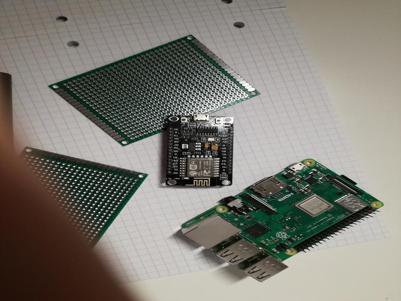
This tutorial uses the Microcontroller Object Detection dataset, which includes images with four models of microcontrollers — ESP8266, Arduino Nano, Heltec ESP32 Lora, and Raspberry Pi 3.

We will build a model that detects whether and where these objects are present in the images, and then labels which microcontrollers are present.

Explore and prepare the data#

Let’s take a closer look at the data before we begin modeling.

Explore the data#

The Flow includes one folder, images, which contains 148 images, and a dataset, annotations, which contains object labels for our model. As with image classification in Dataiku, the images must be stored in managed folders.

To create an object detection model, the images also must be labeled with bounding boxes around the objects of interest. These bounding boxes are represented in a tabular data file that will be input into the model.

Open the annotations dataset.
Right click on a value in the label column.
Select Show complete value or Compare column values side by side to confirm that the label column contains an array of the bounding box coordinates and the target category label for the associated image in the record_id column.

Note

See the reference documentation on the target column format for object detection for more detailed information about the correct formats for images and label inputs for object detection.

If your images are annotated in Pascal or VOC format you can use the plugin Image Annotations to Dataset to reformat the labels.

View the images with bounding boxes#

It is helpful to view the images with their bounding boxes. To do so, you’ll first need to turn on the image view.

Navigate to the Settings tab.
Go to the Advanced subtab.
Scroll down to the Image view section, and select the checkbox Display image view.
Provide the following settings:
- Set the image folder to images.
- Set the path column to record_id.
- Check the box Has annotations.
- Set the annotation column to label.
- Set the annotation type to Object detection.
Click Auto detect classes. You should see all four classes appear.
Click Save.

Now let’s view the images, including the bounding boxes!

Return to the dataset Explore tab of the annotations dataset.
Next to the Table and Columns view, click Images to browse the images including the bounding boxes.
Click on any image to view more information.

Tip

Images can have multiple bounding boxes for images of the same class or even multiple classes.

Create training and testing sets#

Before creating a model, we’ll split the images into training and testing sets, so we can later test how the model performs on images it has never seen.

We’ll do this by splitting the annotations dataset into training and testing datasets, and each of those will point to different sets of images in the image folder.

Open the Actions panel of the annotations dataset.
Select Split from the menu of visual recipes.
Add annotations_train as an output dataset.
Add annotations_test as a second output dataset.
Click Create Recipe.

Now just define the recipe’s configuration.

In the recipe’s settings, select Randomly dispatch data as the splitting method.
Send 80 % of the data into annotations_train, leaving the other 20% in annotations_test.
Click Run to execute the recipe.

Fine-tune a pre-trained object detection model#

After exploring and splitting the data, we are ready to use the pre-trained object detection model in Dataiku.

Create an object detection task#

In this section, we’ll create a model in the Lab, and later we’ll deploy it in the Flow to test it on new images.

In the Flow, select the annotations_train dataset.
Navigate to the Lab in the right panel.
Select Object Detection as the visual ML task.
Select label as the model’s target, or what objects it will detect and classes it will predict.
Select images as the image folder where training images should be found.
Click Create.

Review the model’s target and test split#

Before training the model in the Lab, let’s review the input and settings in the Design tab.

In the Basic > Target panel, confirm the selections for the target column, path column, and image location.
Under Target classes, filter the four automatically-detected classes, and click on a few images to browse the training data.
Confirm the settings in the Train / Test Set panel.

Dataiku automatically split the images into training and validation sets so the model can continually test its performance during the training phase.

Tip

The Train / Test Set panel also contains sampling settings, which you might want to change when using larger datasets!

Review the model’s training settings#

In the Training panel, you’ll find the settings for fine-tuning the pre-trained model. There is only one potential model to use — the Faster R-CNN, which is a faster-performing iteration of a neural network model that divides images into regions to detect objects more quickly.

Navigate to the Training panel.
Confirm Faster R-CNN is selected as the pre-trained model.
Confirm that 0 fine-tuned layers will be used. See the note below for details.
Confirm Early stopping is selected so that the training of the model finishes quicker.
Set Early stopping patience to 3 so that the model will stop cycling through images if it does not detect any performance improvement after three cycles, or epochs.

Important

Convolutional neural networks (CNN) have many different layers that are pre-trained on millions of images.

Retraining the final layer or final few layers helps the model learn on your specific images. Dataiku’s models always retrain the final layer, also called the classifier layer, to adapt it to the use case at hand.

The default setting of 0 under Number of fine-tuned layers means one layer will be fine-tuned. Inputting 1 here would mean that two layers will be fine-tuned, and so on. Adding fine-tuned layers can increase performance, but also increases processing time.

Values for the Optimization and Fine-tuning sections are set to industry standards, and in most cases you will not change these.

Review the runtime environment#

Even with the relatively small set of images used for this tutorial, training an image classification or object detection model can take a long time. Without GPUs, the model training task here might take 30 to 90 minutes.

For real use cases, if your Dataiku instance is running on a server with a GPU, you can activate the GPU for training so the model can process much more quickly. Otherwise, the model will run on CPU, and the training will take longer. You may also execute the training in a container.

Navigate to the Advanced > Runtime environment panel.
Confirm a compatible code environment is selected, as described in the tutorial prerequisites.
If available, consider executing the model training in a container or activating GPUs.

Tip

If you are using Dataiku Cloud, for the purpose of this tutorial, you may want to select a container configuration, such as CPU-S-0.5-cpu-2Gb-Ram.

Train the model#

When you are finished adjusting the model’s design, it’s time to train!

Click Train at the top right to begin training the model.
In the window, give your model a name or use the default, and select Train once more.

Interpret model metrics and explainability#

After training completes, you can assess the performance of a model before deploying it to the Flow.

View the model summary#

Unlike with an AutoML prediction task, we only have one candidate model to review.

From the Result tab, click on the model name to navigate to the model report.
Read the Summary panel for an overview of the model’s training information, including the classes, epochs trained, and other parameters.
Navigate to the Training information panel for model diagnostics, runtime configuration, and validation strategy.

Submit a new image#

You can upload new images directly into the model to find objects and view the probabilities of each detected class. This information can give you insight into how the algorithm works and potential ways to improve it.

To see how this works, we’ll input a new image our model has not seen before.

Download the file microcontroller_what-if, which is an image that contains two controllers — a Raspberry Pi and a ESP8266.
In the model report, navigate to What if? panel.
Either drag and drop the new image onto the screen, or click Browse For Images and find the image to upload.
The model should detect both a Raspberry Pi and an ESP microcontroller. We also do not see any false positive detections on other objects in the image.
Hover over the class names on the right to highlight the objects detected in the image.

Interpret the confusion matrix#

Dataiku calculates the number of true positive and false positive detections in the testing set of images, and then inputs those values into a confusion matrix.

Under Explainability, navigate to the Confusion matrix panel.
Confirm the number of true positives for each microcontroller along the matrix’s diagonal. This diagonal reports where the model correctly detected the objects found in the images.
Filter the images displayed on the right by clicking on any value in the confusion matrix, such as the value where the model correctly predicted a Raspberry Pi.
Double click on any image on the right to view the ground truth and predicted object bounding boxes, the object class, and confidence level.

The true and false positive calculations in the confusion matrix are based on two measures: the Intersection over union (IOU) and the Confidence score.

The Confidence score is the probability that a predicted box contains the predicted object.
IOU is a measure of the overlap between the model’s predicted bounding box and the ground truth bounding box provided in the training images. By comparing the IOU to an overlap threshold that you set, Dataiku can tell if a detection is correct (a true positive), incorrect (a false positive), or completely missed (a false negative).

The IOU threshold is the lowest acceptable overlap for a detection to be considered a true positive. For example, with a threshold of 50%, the model’s detected object must overlap the true object by 50% or more to be considered a true detection. If a detection overlaps by only 40%, it would be considered a false positive.

Let’s experiment with different settings and now how the values in the matrix change.

Above the confusion matrix, increase the IOU to 0.75.
Increase the Confidence score to 0.75.
Observe how more records fall into the Not Detected column of the matrix.
Click Revert to Optimal when finished.

Analyze performance#

The evaluation metric is Average precision, which measures how well your model performs. The closer to 1 this score is, the better your model is performing on the test set.

Under Performance, navigate to the Metrics panel.
Find the microcontroller that the model did the best job of detecting. In our case, it is Heltec ESP32 Lora.
Confirm that the model’s performance declines as the IOU increases from 0.5 to 0.75 because the overlap threshold for counting a true positive detection is higher.
The average precision measures the area under the precision-recall curve. Navigate to the Precision-Recall panel, and read the graphic to understand its interpretation.

Test the object detection model#

Now that we have reviewed performance of the model, we can deploy it from the Lab to the Flow so we can use it to detect objects in new images (or further test the performance of the model, as is the case here).

Deploy the model to the Flow#

Deploying a model from the Lab to the Flow is just like any other visual model.

From the model report, click Deploy in the top right corner.
Click Create, and find the training recipe and model added to the Flow.

Tip

You can find a model in the Lab at any time in two ways:

The Visual Analyses menu (g + a) in the top navigation bar.
The training dataset’s Lab tab in the right panel in the Flow.

Detect objects in new images#

We can now use the model to make detect objects in images held aside in the annotations_test dataset.

Important

Although all images for this project are found in the same images folder, only the records in the annotations_train dataset were actually sent to the model for training. The model has not yet seen the images described in the annotations_test dataset, even though they also reside in the images folder.

From the Flow, select the saved model and the annotations_test dataset.
In the right panel, select Score.
Under Inputs, select images as the managed folder containing the images.
Click Create Recipe.
On the recipe’s Settings tab, leave the default batch size of 2, and click Run to execute the recipe.
When the recipe finishes running, open the dataset annotations_test_scored.

Note

The Score recipe’s Settings tab lets you change the batch size, edit how many images to score at a time, or activate GPU to run scoring more quickly if that is available to you.

Explore the scored image output#

When exploring the annotations_test_scored dataset, you’ll notice that in addition to the usual table and columns view, there is also a view for images.

While in the Images view of the Explore tab, browse through some images to see the prediction categories compared to their true label values.
Switch to the Table view.
Observe the new prediction column, including an array of the bounding box, category, and confidence level for any detected objects.
Right click on a value in the label column, and select Compare column values side by side.
Select prediction as the column for comparison.
Browse through the results, noting that in some cases the model detects multiple classes for a single object.

Tip

If the prediction column is empty, that means the model did not detect an object in those images.

What’s next?#

Congratulations on building your first object detection model in Dataiku! You’re ready to create a new model on your own images.