
Concept | Time series windowing#
An overview of time series windowing#
You might be familiar with the native Window recipe in Dataiku.
Let’s draw on your knowledge of this recipe to understand the Windowing recipe of the Time Series Preparation plugin, which is specifically geared to work with time series data.
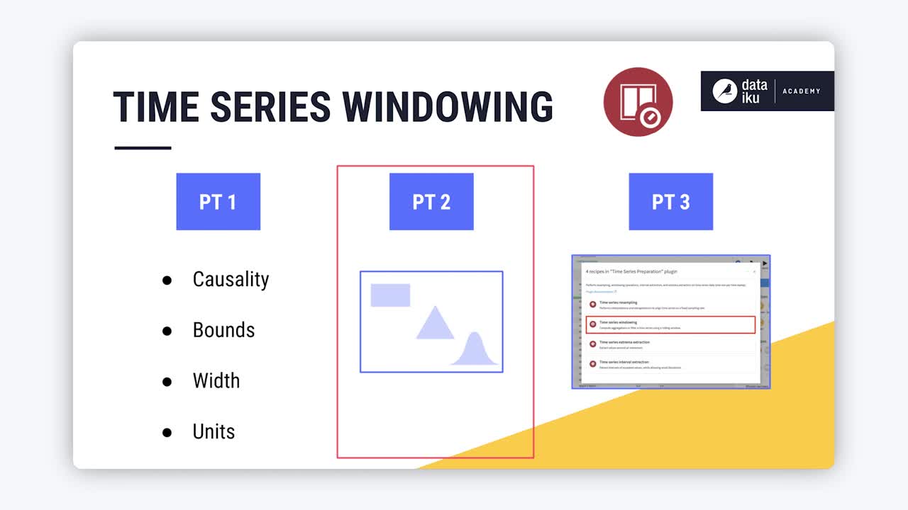
Using this recipe requires understanding a few different parameters, so we’ve divided this article into three parts:
Introducing parameters like causality, bounds, width, and units.
Understanding the concept of window shape.
Walking through a demo using the recipe.

An introduction to time series windowing parameters#
Watch the video or read the summary below.

Visual Window recipe recap#
Let’s begin by reminding ourselves how to define window frames using the visual Window recipe.

In this example, we only have a single time series, so we don’t need to worry about partitioning columns.
We can order rows by the date column in an increasing order.
Then, we choose the rows to include in the window frame. Here we include 1 preceding row and 0 rows after the current row.
Once the window frame is set, we choose an aggregation, like a sum.
Then, starting from the beginning, Dataiku works its way down and calculates the aggregation row by row.
Time series windowing parameters#
We can recreate this output with the time series Windowing recipe. You haven’t seen these parameters before, but they come directly from the dialog of the time series Windowing recipe.

You’ll need to become familiar with terms like:
Causality
Shape
Width
Units
Bounds
Causality#
Let’s start with causality. In the time series windowing recipe, we first have to decide whether to build a causal or non-causal window.
A causal window can only include past values and/or the current value in the window frame. It can’t include future values.
A non-causal window (also known as a bilateral window) can include past, current, and future values.

The previous example using the visual Window recipe implemented a causal window frame because it included only past and current values.
Causality is important because it defines the relationship between the current row and the window frame.
In a causal window, the current row is always at the right bound of the window frame.
In a non-causal window, the current row is at or near the midpoint of the window frame, depending on whether the width is odd or even.

We’ll see how this works below.
Bounds#
You can think of bounds as the boundary or the edge of the window frame.

In a causal window frame, if 2020-07-02 is our current row, that makes 2020-07-02 the right bound. Knowing the right bound of a causal window is simple. It’s always the current row.
The left bound is determined by two more parameters: width and units. We can think of the right bound as row zero and move back in time to set the left bound according to the width.
Since the width of this window frame is 1 day, if 2020-07-02 is the right bound, then the left bound must be one day prior, 2020-07-01 or July 1.
It’s easier to see where the names for left and right bounds come from when looking at a line plot.

The right bound is the current timestamp, and the left bound is the earliest timestamp.
Once we have the placement of left and right bounds, we always have the option of whether to include or exclude them from the aggregation.
By default, the left bound is included in the aggregation, and the right bound, despite being part of the window frame, is excluded from any requested aggregations. This means, by default, the causal window frame in the Windowing recipe includes only past values.
In this example though, we’re including both window bounds.

Window shape#
One remaining parameter needed to define a window frame is shape.
By selecting a rectangular window, all the values in the window are weighted equally, just as in the visual Window recipe. We’ll discuss the concept of window shape in more detail later in this summary.

Window aggregations#
Now that we have a handle on causality, shape, width, units, and bounds, we can finally configure the aggregations.
Retrieve allows us to return the original column of values in the output, and Sum returns a column containing the sum of values in the window frame for each row.
We then slide down the dataset row by row, returning the requested aggregations, just like with the visual Window recipe.

Adjusting time series windowing parameters#
Now we have fully reproduced the example originally computed with the visual Window recipe, by using the time series Windowing recipe.

Let’s start adjusting some of these parameters to get a better feel for how they work.
Increasing width#
Let’s keep all these parameters the same, but increase the width of the window frame from 1 to 2 days. What do we expect will happen?
Because this is a causal window, the right bound remains positioned at the current date. We only need to find the left bound.
If the width is
2, we count two days instead of one.If the width was
3, we count three days before the current day.

Notice how we said three days instead of three rows. In this example, previous days and previous rows are the same, but this might not always be the case if some sequential dates are missing.
Changing window units#
We’re speaking in terms of days for this example, but depending on our data, this could be units as large as years or as small as nanoseconds.

Including/excluding bounds#
Let’s finish the aggregation for this window frame. We have four values in a causal window frame of three days. From here, we can choose to:
Include both left and right bounds and sum all four values.
Include only the left bound.
Include only the right bound.
Include neither bounds.

Changing aggregations#
Once we have the window frame defined, we can always change the aggregation. For example, we could change the aggregation from a rolling sum to a rolling average.

We could also choose from many other options, such as the median.

Non-causal windows#
We can build a non-causal or bilateral window by un-checking the causal window parameter.
Recall that, in a non-causal window, the current row is at or near the midpoint of the window frame instead of the right bound.
Once the causal box is unchecked, we no longer have the option to include or exclude the window bounds. Instead, we only have to think about the width.
If we start with a non-causal window and a width of one day, our average is just the current value. But as we increase the window width, what’s happening becomes clear.

We’re able to include values from both past and future timestamps in the window frame, centered around the current timestamp.
When we have an odd width like
3, it’s easy to place the current row at the midpoint of the window frame.When we have an even width like
4, the midpoint lies between two timestamps. We always choose the more recent one.At an odd width like
5, we’ll include two past values, the current value, and two future values.
Window units#
Thus far, we haven’t talked much about the units attached to the width of the window frame. But this is an important feature of the time series Windowing recipe not found in the visual Window recipe.
Imagine expanding a non-causal window from 5 to 7 days. This would give us a rolling weekly average in this case. We could achieve the same results by setting the width to one week instead of seven days.
Imagine though, if we had a larger time series, where we wanted the width of the window to be a month or a year. On the orders dataset, we can see how adjusting the window frame units from days to weeks to months to years smooths out the trend on a line plot.

Time series window shape#
Watch the video or read the summary below.
At this point, we have talked about causality, width, units, bounds, and aggregations. That leaves only shape. The shape of the window frame in all previous examples is a rectangle. What does this parameter mean?

Rectangular window frames#
Consider a causal window of two days, including both left and right bounds in the aggregations. When calculating the rolling sum, it made no difference if a value was positioned at the beginning, middle, or end of the window frame.
In other words, we can think of all values in the rectangular window frame as having a weight of 1.
Two new columns in the table, weight and weighted revenue, will help us think through the shape parameter.
Dataiku assigns a weight of
1to all values contained in the rectangular window frame.If we multiply all the original values by their weight of
1, we of course get the same output.We can then proceed with our aggregations in the same way as before, using the weighted revenue instead of the original revenue values.

Let’s take a graphical approach. We can visualize a rectangular shape if we draw the horizontal width the same width as the window frame and assign a uniform vertical length of 1.

When we multiply each observation in the original line plot by its assigned weight, the weighted revenue is identical to the original revenue values.
Remember though that time series don’t consist of independent observations. Perhaps we don’t want to give equal weights to all values in the window frame. In some cases, we may want values in the center of the window frame to be of greater importance than those values on the edges.
Triangular window frames#
We can imagine weighting the values in a window frame according to shapes other than a simple rectangle, such as a triangle, or a variety of other bell-shaped curves.
Let’s walk through this again with a new example. Below we have a non-causal window.
We will start with a width of one day and watch it expand into both past and future values, centered around the present. Instead of the usual rectangular window though, let’s make it a triangular window.

With a width of just one day, our results are the same as we’d find for a rectangular window. The weight can only be 1.
What happens to the weights as the width of the window frame expands? The general idea is to first find the center of the window frame. With an even width, the center falls between two rows. The center of the window frame will be the center of the triangle.
Think of the peak of the triangle as having a weight of 1. Then the weights decrease moving out toward the ends of the window frame. In a triangle window, that decrease is linear, making each row equally weighted at 0.5.
Applying these weights, we get our weighted revenue. From the weighted values, we can now calculate the aggregation as we normally would, in this case, a sum.
Let’s expand the width to three days, keeping all the other parameters the same. First find the center. For a non-causal window of an odd width, that’s the current timestamp. Assign the center of the window frame a weight of 1. Now decrease the weights linearly moving out from the center. Then just like before, sum the weighted values to get the final result.
We can see this trend continue as we move to a width of four days. Find the center. Assign the weights based on the chosen shape. Use the weighted values to perform the requested aggregation.
For now, let’s stop at a width of five days and instead see what’s happening on the line plot. As the width of the window frame increases, we can see how the weights assigned by the triangle change.
At the same time, we can plot the weighted revenue, the result of multiplying the original values by their assigned weight.

Shape as a function#
Having seen a few simple examples, you can begin to see that the shape parameter is just a function.
The original values in your time series are the inputs to the shape function.
The shape function assigns weights to these time series values based on the chosen shape and other window parameters like width and bounds.
After passing through the shape function, we have weighted values as output.

It’s these weighted values that will get passed to the aggregation step, like a rolling sum or an average.

If the window shape is a rectangle, this function is simple. All weights are just 1. If the shape is a triangle, the weights start at 1 in the center and decrease linearly.
However, the shape function can be something more complex. The recipe makes it possible to assign weights according to a number of different bell-shaped curves.

Demo#
Watch the video or read the summary below.

Now that you know how parameters like causality, shape, width, units, and bounds all work together to define a window frame, actually doing so in Dataiku should be easy. That’s what we’ll cover next.

Using the time series windowing recipe#
Let’s return to our familiar t-shirt orders data.
What do we need from our data to use the time series Windowing recipe?
Like all other recipes in the plugin, we need a valid time series with a parsed date column.
Unlike the Resampling recipe though, if we have multiple time series in the dataset, then the data must be stored in the long format.
The data doesn’t necessarily need to be resampled to run the time series Windowing recipe, but you should be careful about failing to do so.
This is because, if timestamps aren’t equispaced, or if your data is missing some required interpolation or extrapolation steps, the output of the Windowing recipe may not represent what you expect.
For the input to the Windowing recipe, let’s use the resampled, long format time series, where we interpolated a constant value of 0 for dates with no sales. From this dataset, we’re ready to build any kind of windows we need.

As with all recipes in the plugin, we first provide the name of the timestamp column.
We also know the data is in long format, with the tshirt_category column serving as the identifier column.
The Window parameters should look quite familiar by now.
You should experiment on your own by building different kinds of windows, but for now let’s build a causal, rectangular window of three days, including only the left bound.
We’ll retrieve our measurements, calculate the average, and find the sum using a rolling window.

In the output, observe that the numerical columns from the input dataset have been retrieved along with the timestamp and the identifier columns.
In addition, for each of the numerical columns, there are two new columns, one for each of the aggregates (average and sum).

The results are sorted first by the identifier column groups, and then in ascending order by date.
Now it’s up to you to build your own windows that achieve your time series goals!
Next steps#
Congratulations! Once you have a handle on time series windowing, learn how the same knowledge of building window frames can be used in the Extrema Extraction recipe.